Gradient Descent from scratch and visualization
Gradient descent is an optimization algorithm used to minimize some function by iteratively moving in the direction of steepest descent as defined by the negative of the gradient. In machine learning, we use gradient descent to update the parameters of our model. Parameters refer to coefficients in Linear Regression and weights in neural networks.
Below video discusses about gradient descent algorithm. Its good to spend some time on this video and get intuition about it before we start writing code for it.
library(ggplot2)
library(dplyr)
library(magrittr)
library(Deriv)
library(gganimate)

# define the function we want to optimize
#f <- function(x) ((x^2-4*x+4)*(x^2+4*x+2))

f <-  function(x) {
  1.2 * (x-2)^2 + 3.2
}

#define the cost function
cost <- Deriv(f)


#Gradient Descent Implementation
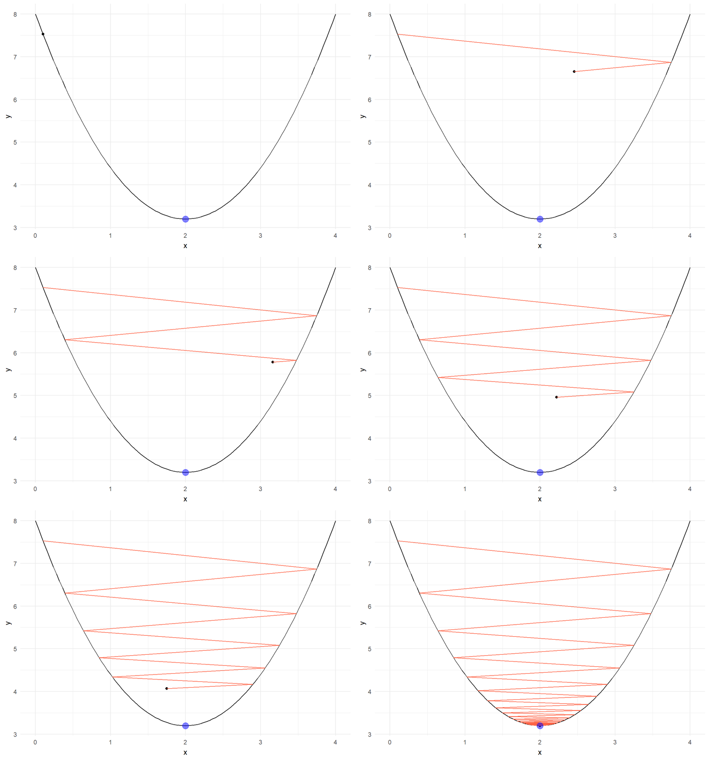
grad <- function(x = 0.1, alpha = 0.8, j = 100) {
  xtrace <- x
  ftrace <- f(x)
  for (i in 1:j) {

    x <- x - alpha * cost(x)
    xtrace <- c(xtrace,x)
    ftrace <- c(ftrace,f(x))
  }
  return(data.frame( "x" = xtrace,
                     "f_x" = ftrace))
}
#grad()


val <- grad()
val %>% mutate(id = row_number())->val
i = length(val$x)

x_on_iteration_i <- val$x[i]
y_on_iteration_i <- val$f_x[i]


  ggplot(data = data.frame(x = 0), mapping = aes(x=x))+
  stat_function(fun = f) +
  xlim(0,4)+
  geom_point(data = val, aes(x, f_x))+
  geom_path(data = val, aes(x, f_x), color = "tomato")+
  geom_point(x = x_on_iteration_i, y = y_on_iteration_i, color = 'blue', size = 4, alpha = 0.5)+
  theme(legend.position="none")+
  transition_reveal(along = -f_x)+
  theme_minimal()
