Hypothesis Testing made simple
In this post we will use a very elegant and simple approach to test any hypothesis. This approach is based on growing trend of emphasizing data and simulations instead of classical probability theory and complex statistical tests. Since We know that its hard to wrap the head around how to reject null hypotheses and interpret p-values.
The new approach however has this philosphy that there is only one statistical test and that at their core, all statistical tests (be they t-tests, chi-squared tests, signed Wilcoxon rank tests, etc.) follow the same universal pattern.
So here is the framework for conducting any hypothetical test :-
Step 1 :-
Calculate the sample statistic (e.g. difference in means, average, median, proportions, difference in proportions, chi-square value). This is basically statistic from observed data.
Step 2 :-
Now you define your null hypothesis and simulate a world for the null hypothesis. For example, if you think there might be a difference between two groups, the null hypothesis would assume that there is no difference.
Note:- Your model of the null hypothesis should be capable of generating random datasets similar to the original dataset.
Step 3 :-
After that compute the same sample statistic for your simulated datasets.
Step 4 :-
Calculate the probability (i.e. p-value) that sample statistic could exist in null world i.e. Count the fraction of times the sample statistic from simulated datasets exceed sample statistic from observed data. This fraction is approximates the p-value.
Step 5 :-
Decide if sample statistic is statistically significant by choosing some thresholds. Some thresholds are (from least to rigorous) 0.1 , 0.05, 0.01
If it’s sufficiently small, you can conclude that the apparent effect is unlikely to be due to chance.
Statistical Significant simply means that the result we see in the sample also exists in the population and hence statistic is reliable.
These are the only 5 steps we need to test any hypothesis no need to remember any flowchart or the statistical test.
Specify Statistic –> Generate Data –> Calculate Statistic —> Visualize
We will use infer package for the above framework. Below are the important functions of this package:-
specify:- the response and explanatory variable(y~x)
hypothesize:- what the null hypothesis is ?
generate:- Generate new samples under the null hypothesis model.
resample from our original data without replacement, each time shuffling thegroup(type = "permute")
calculate:- the statistic(stat = "diff in props")for each of the reps.
visualize:- for visualization
Now let’s take an example
Question:- Is an automatic or manual transmission better for mpg ?
Dataset
library(tidyverse)
library(ggridges)
library(scales)
library(infer)
set.seed(123) #To make random draws reproducible
mtcars %>% mutate(type = ifelse(am == 1, "manual", "automatic")) %>% glimpse() ->mtcars_dataset
## Observations: 32
## Variables: 12
## $ mpg <dbl> 21.0, 21.0, 22.8, 21.4, 18.7, 18.1, 14.3, 24.4, 22.8, 19.2,…
## $ cyl <dbl> 6, 6, 4, 6, 8, 6, 8, 4, 4, 6, 6, 8, 8, 8, 8, 8, 8, 4, 4, 4,…
## $ disp <dbl> 160.0, 160.0, 108.0, 258.0, 360.0, 225.0, 360.0, 146.7, 140…
## $ hp <dbl> 110, 110, 93, 110, 175, 105, 245, 62, 95, 123, 123, 180, 18…
## $ drat <dbl> 3.90, 3.90, 3.85, 3.08, 3.15, 2.76, 3.21, 3.69, 3.92, 3.92,…
## $ wt <dbl> 2.620, 2.875, 2.320, 3.215, 3.440, 3.460, 3.570, 3.190, 3.1…
## $ qsec <dbl> 16.46, 17.02, 18.61, 19.44, 17.02, 20.22, 15.84, 20.00, 22.…
## $ vs <dbl> 0, 0, 1, 1, 0, 1, 0, 1, 1, 1, 1, 0, 0, 0, 0, 0, 0, 1, 1, 1,…
## $ am <dbl> 1, 1, 1, 0, 0, 0, 0, 0, 0, 0, 0, 0, 0, 0, 0, 0, 0, 1, 1, 1,…
## $ gear <dbl> 4, 4, 4, 3, 3, 3, 3, 4, 4, 4, 4, 3, 3, 3, 3, 3, 3, 4, 4, 4,…
## $ carb <dbl> 4, 4, 1, 1, 2, 1, 4, 2, 2, 4, 4, 3, 3, 3, 4, 4, 4, 1, 2, 1,…
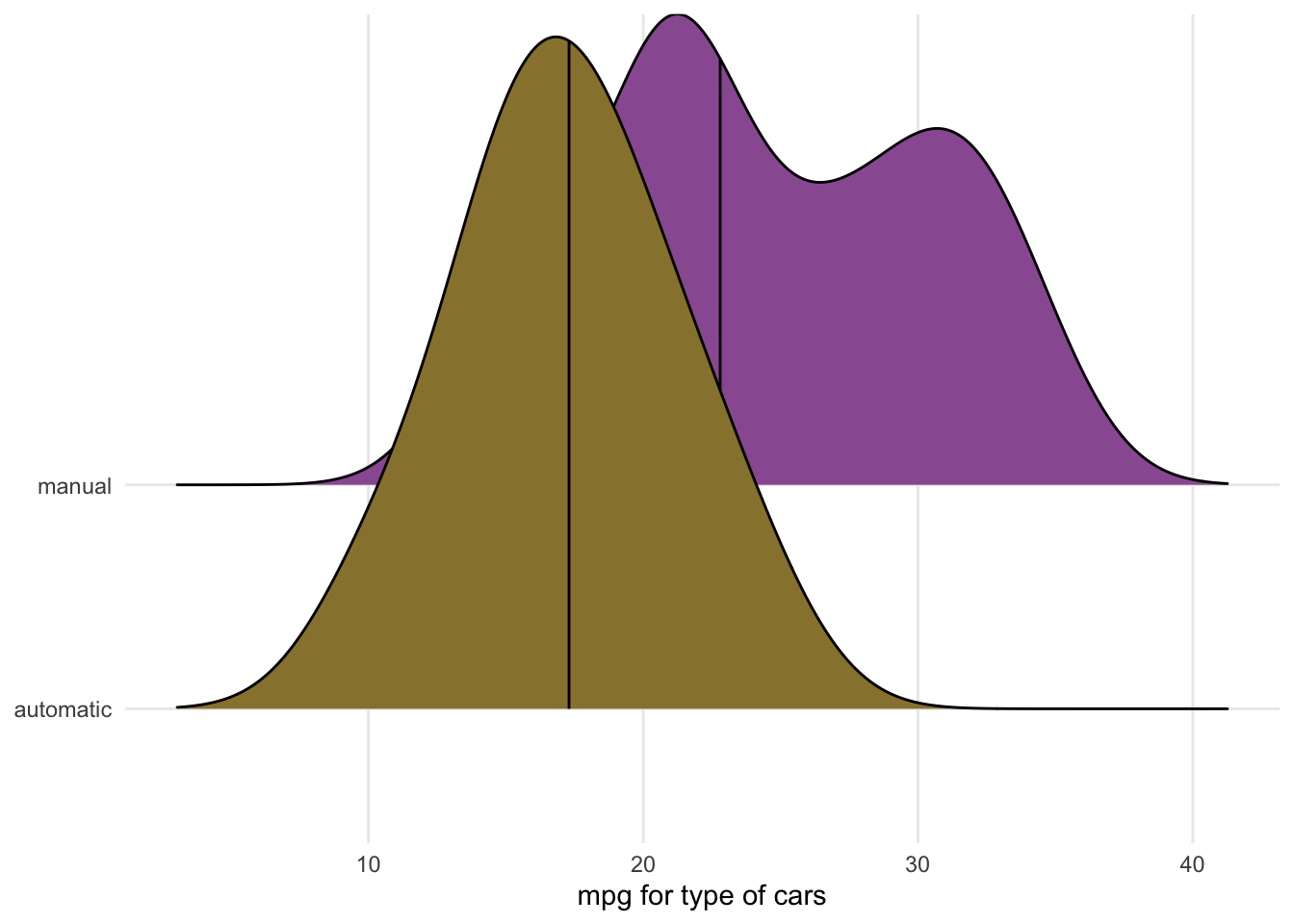
## $ type <chr> "manual", "manual", "manual", "automatic", "automatic", "au…First we just look at the ridge plot to see if there is a differnce in distribution of car_type in automatic and manual. We include quantile_lines = TRUE and quantiles = 2 to draw the median of each distribution.
ggplot(mtcars_dataset, aes(x = mpg, y = type, fill = type)) +
  stat_density_ridges(quantile_lines = TRUE, quantiles = 2, scale = 3, color = "black") +
  scale_fill_manual(values = c("#98823c", "#9a5ea1"), guide = FALSE) +
  labs(x = "mpg for type of cars", y = NULL) +
  theme_minimal() +
  theme(panel.grid.minor = element_blank())
Null Hypothesis :- The median of mpg of automatic and manual transmission cars are same.
Step 1: -
We can use the infer package to determine the exact difference in the medians of these distributions.
(diff_prop <- mtcars_dataset %>%
  specify(mpg~type) %>%
  calculate("diff in medians",
            order = c("manual", "automatic")))
## # A tibble: 1 x 1
## stat
## <dbl>
## 1 5.55.5 is our sample statistic value.
The question is whether this difference is statistically significant?
Step 2 and 3 :-
Simulate the world where the actual difference between the automatic and manual car is zero and calculate the sample statistic for each simulated dataset.
mtcars_null_dataset <- mtcars_dataset %>%
  specify(mpg~type) %>%
  hypothesize(null = "independence") %>%
  generate(reps = 5000) %>%
  calculate("diff in medians", order = c("manual", "automatic"))
Step 4 :-
mtcars_null_dataset %>%
  visualize(obs_stat = diff_prop)+
  theme_minimal()+
  theme(panel.grid.minor = element_blank())
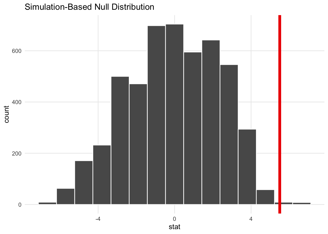
Note that red line is pretty far in the right tail of the distribution and seems atypical. We can calculate the probability of seeing a difference as big as 5.5 with the get_pvalue() function.
Here we specify the direction = "both" to get two tailed p-value since we care about only the difference between mean or median(as difference could be negative if flip the order).
mtcars_null_dataset %>%
  get_pvalue(obs_stat = diff_prop, direction = "both")
## # A tibble: 1 x 1
## p_value
## <dbl>
## 1 0.0068Step 5:-
The point here is that there is only 0.68% of chance of seeing a difference at least as large as 5.5 in a world there is no difference. Its pretty strong evidence and we feel confident that there’s a statistically significant difference between mpg of automatic and manual where manual cars give more mpg than automatic cars.
