Learn Machine Learning using Kaggle Competition titanic 🚢 dataset
This post is an effort of showing an approach of Machine learning in R using tidyverse and tidymodels. We will go through step by step from data import to final model evaluation process in machine learning. We will not just focus on coding part but also the statistical aspect should be taken into account behind the modelling process. In this tutorial we are using titanic dataset from Kaggle competition.
Modelling Process and packages involves :-
In R we can use following tidyverse packages to make machine learning model process streamline.
- Data import/export :- readr
- Exploratory Data Analysis (Data cleaning and exploration and visualization) : tidyverse
- Resampling (e.g. Bootstrap,Cross Validation) and Parameter tuning :- rsample
- Preprocessing and feature engineering :- recipes
- Model building :- parsnip
- Model evaluation :- yardstick
Table of Contents :-
Titanic: Machine Learning from Disaster
1. Understanding Business Problem
The very step in a machine learning project to understand the business problem we are trying to solve.Get the domain knowledge and look for the metrics which can help in solving that problem.
Consider a business problem of measuring the customer loyalty since it is not measurable quantity we can look for metric like Net Promoter Score which captures this.
In our problem we need to find survival chances of an individual on the titanic. The feature i.e. Survived tells us whether the particular individual survived or not.Its very simple to determine in this case since its toy dataset problem. However real world business problems are more complex and need more brainstorming session to convert a business problem into analytical problem.
2. Hypothesis Generation
During hypothesis generation we create a set of features which could impact the target variable.We should do this before getting the data so as to avoid the biased thoughts. This step also help in creating new features.
Some of factor which I think of that directly influence the target variable as i know this disaster is famous for saving women and children first :-
- Sex
- Age
- Fare
- Ticket Class
- Travelling with or without family
3. Setup and Data import
Next thing is to setup your path to the location where data is stored and then import dataset into R. We will use readr package of tidyverse family to read data into R. There are some other packages as well which read csv data faster than readr package. Some of them are:- data.table and Vroom
Since we are not dealing with very huge amount of data we don’t require to load those package for this tutorial. But when size of csv goes greater than 2 gb or so you should refer vroom and data.table.
Loading libraries and Setting up path
setwd("D:/kaggle/titanic")
library(tidymodels) #for modelling
library(tidyverse)  # for data cleaning and processing
library(gridExtra)  # for plotting multiple graphs
library(mice)       # for missing value treatment
library(moments)    # for calculating skewness and kurtosis
library(outliers)   # for outlier detection
library(gganimate) # for animationYou can download the dataset from here. I stored the dataset in my D drive in titanic folder which is inside the kaggle folder and hence provided that path for data reading.
train <- readr::read_csv("train.csv")
test <- readr::read_csv("test.csv")
Setting theme for visualization
mytheme <- function(...){
                 theme(legend.position = "bottom",
                 legend.text = element_text(size = 8),
                 panel.background = element_rect(fill = "white"),
                 strip.background = element_rect(fill = "white"),
                 axis.line.x = element_line(color="black"),
                 axis.line.y = element_line(color="black"))
}
4. Exploratory Data Analysis
Exploratory Data Analysis in short known as EDA is way of summarizing, interpreting and visualizing the information hidden in rows and column format. Simply EDA is the key to getting insights from data.
Why EDA is important ?
Usually we start any data science project with understanding the business problem and then we genrate hypothesis. During hypothesis generation we look for factors which influence our dependent variable. EDA helps in confirming and validating those hypothesis.
It helps to find out unexpected pattern in data which must be taken into account, thereby suggesting some changes in planned analysis.
Deliver data driven insights to business stakeholders by confirming they are asking the right questions and not biasing the investigation with their assumptions.
Practitioners say a good data exploration strategy can solve even complicated problems in a few hours.
The first step of EDA is Variable identification here we identify Predictor (Input) and Target (Output) Variables. Also we identify datatype and category of the variables.
#Check the dimension of test and train dataset
cat("There are ", dim(train)[1], "rows and ",dim(train)[2],"columns in train dataset")
## There are 891 rows and 12 columns in train datasetcat("There are ", dim(test)[1], "rows and ",dim(test)[2],"columns in test dataset")## There are 418 rows and 11 columns in test datasetLets see variables in train set and thier datatype
train %>%
  glimpse()
## Observations: 891
## Variables: 12
## $ PassengerId <dbl> 1, 2, 3, 4, 5, 6, 7, 8, 9, 10, 11, 12, 13, 14, 15,...
## $ Survived <dbl> 0, 1, 1, 1, 0, 0, 0, 0, 1, 1, 1, 1, 0, 0, 0, 1, 0,...
## $ Pclass <dbl> 3, 1, 3, 1, 3, 3, 1, 3, 3, 2, 3, 1, 3, 3, 3, 2, 3,...
## $ Name <chr> "Braund, Mr. Owen Harris", "Cumings, Mrs. John Bra...
## $ Sex <chr> "male", "female", "female", "female", "male", "mal...
## $ Age <dbl> 22, 38, 26, 35, 35, NA, 54, 2, 27, 14, 4, 58, 20, ...
## $ SibSp <dbl> 1, 1, 0, 1, 0, 0, 0, 3, 0, 1, 1, 0, 0, 1, 0, 0, 4,...
## $ Parch <dbl> 0, 0, 0, 0, 0, 0, 0, 1, 2, 0, 1, 0, 0, 5, 0, 0, 1,...
## $ Ticket <chr> "A/5 21171", "PC 17599", "STON/O2. 3101282", "1138...
## $ Fare <dbl> 7.2500, 71.2833, 7.9250, 53.1000, 8.0500, 8.4583, ...
## $ Cabin <chr> NA, "C85", NA, "C123", NA, NA, "E46", NA, NA, NA, ...
## $ Embarked <chr> "S", "C", "S", "S", "S", "Q", "S", "S", "S", "C", ...Now Lets see variable in test set and their datatypes
test %>%
  glimpse()
## Observations: 418
## Variables: 11
## $ PassengerId <dbl> 892, 893, 894, 895, 896, 897, 898, 899, 900, 901, ...
## $ Pclass <dbl> 3, 3, 2, 3, 3, 3, 3, 2, 3, 3, 3, 1, 1, 2, 1, 2, 2,...
## $ Name <chr> "Kelly, Mr. James", "Wilkes, Mrs. James (Ellen Nee...
## $ Sex <chr> "male", "female", "male", "male", "female", "male"...
## $ Age <dbl> 34.5, 47.0, 62.0, 27.0, 22.0, 14.0, 30.0, 26.0, 18...
## $ SibSp <dbl> 0, 1, 0, 0, 1, 0, 0, 1, 0, 2, 0, 0, 1, 1, 1, 1, 0,...
## $ Parch <dbl> 0, 0, 0, 0, 1, 0, 0, 1, 0, 0, 0, 0, 0, 0, 0, 0, 0,...
## $ Ticket <chr> "330911", "363272", "240276", "315154", "3101298",...
## $ Fare <dbl> 7.8292, 7.0000, 9.6875, 8.6625, 12.2875, 9.2250, 7...
## $ Cabin <chr> NA, NA, NA, NA, NA, NA, NA, NA, NA, NA, NA, NA, "B...
## $ Embarked <chr> "Q", "S", "Q", "S", "S", "S", "Q", "S", "C", "S", ...For exploratory data analysis and feature engineering we need complete dataset. So lets combined the train and test dataset
df <- bind_rows(train, test)Observations :-
- Variable not present in our test dataset is Target variable i.e. Survived. Whether the passenger survived or not.
- All Other Variables are predictor Variables.
- Here the problem is a classification problem since we have to predicted whether the passenger will survive or not.
In univariate analysis stage we explore each variables one by one. Now the method to do univariate analysis depend on variable type.
- Continuos Variable
- Categorical Variable
Before that lets first convert Pclass, Embarked, Survived and Sex into factors this will better represent different levels and drop passengerid as it is not required.
df %>%
  mutate(Pclass = factor(Pclass),
         Embarked = factor(Embarked),
         Survived = factor(Survived),
         Sex = factor(Sex))->  df
df$PassengerId <- NULL
df %>% glimpse()
## Observations: 1,309
## Variables: 11
## $ Survived <fct> 0, 1, 1, 1, 0, 0, 0, 0, 1, 1, 1, 1, 0, 0, 0, 1, 0, 1,...
## $ Pclass <fct> 3, 1, 3, 1, 3, 3, 1, 3, 3, 2, 3, 1, 3, 3, 3, 2, 3, 2,...
## $ Name <chr> "Braund, Mr. Owen Harris", "Cumings, Mrs. John Bradle...
## $ Sex <fct> male, female, female, female, male, male, male, male,...
## $ Age <dbl> 22, 38, 26, 35, 35, NA, 54, 2, 27, 14, 4, 58, 20, 39,...
## $ SibSp <dbl> 1, 1, 0, 1, 0, 0, 0, 3, 0, 1, 1, 0, 0, 1, 0, 0, 4, 0,...
## $ Parch <dbl> 0, 0, 0, 0, 0, 0, 0, 1, 2, 0, 1, 0, 0, 5, 0, 0, 1, 0,...
## $ Ticket <chr> "A/5 21171", "PC 17599", "STON/O2. 3101282", "113803"...
## $ Fare <dbl> 7.2500, 71.2833, 7.9250, 53.1000, 8.0500, 8.4583, 51....
## $ Cabin <chr> NA, "C85", NA, "C123", NA, NA, "E46", NA, NA, NA, "G6...
## $ Embarked <fct> S, C, S, S, S, Q, S, S, S, C, S, S, S, S, S, S, Q, S,...Univariate Analysis of Continuos variable
Methods used in univariate analysis of continous variable are :-
- Central Tendency -> What are the most typical values ? (Mean Median Mode Min and Max)
- Spread or dispersion -> How do the values vary? (Range Quartile IQR Variance Std.Deviation )
- Shape -> To check the values are symmetrically or assymetrically distributed(Skewness and Kurtosis)
- Outliers : To check abnormalities in the data
- Visualization Methods
#Selecting only continuous variables
num_vars <- df %>%
  select_if(is.numeric)
num_vars %>% glimpse()
## Observations: 1,309
## Variables: 4
## $ Age <dbl> 22, 38, 26, 35, 35, NA, 54, 2, 27, 14, 4, 58, 20, 39, 14...
## $ SibSp <dbl> 1, 1, 0, 1, 0, 0, 0, 3, 0, 1, 1, 0, 0, 1, 0, 0, 4, 0, 1,...
## $ Parch <dbl> 0, 0, 0, 0, 0, 0, 0, 1, 2, 0, 1, 0, 0, 5, 0, 0, 1, 0, 0,...
## $ Fare <dbl> 7.2500, 71.2833, 7.9250, 53.1000, 8.0500, 8.4583, 51.862...Central Tendency
One short way to get the min, mean, median, max and quantiles is using summary function from base package.
summary(num_vars)## Age SibSp Parch Fare
## Min. : 0.17 Min. :0.0000 Min. :0.000 Min. : 0.000
## 1st Qu.:21.00 1st Qu.:0.0000 1st Qu.:0.000 1st Qu.: 7.896
## Median :28.00 Median :0.0000 Median :0.000 Median : 14.454
## Mean :29.88 Mean :0.4989 Mean :0.385 Mean : 33.295
## 3rd Qu.:39.00 3rd Qu.:1.0000 3rd Qu.:0.000 3rd Qu.: 31.275
## Max. :80.00 Max. :8.0000 Max. :9.000 Max. :512.329
## NA's :263 NA's :1summary functions tells us about the central tendency of the variable. However if you want more details summary of variable please check out describe function from Hmisc package. or Psych .Also skimr package is worth checking out.
Unfortunately there is not a built in function to compute mode of a variable.
However we can create a function that takes the vector as an input and gives the mode value as an output:
#Showing as an example
get_mode <- function(v) {
        unique_value <- unique(v)
        unique_value[which.max(tabulate(match(v, unique_value)))]
}
get_mode(num_vars$Fare)
## [1] 8.05Observations from Central Tendency :-
- For Fare mean(33.295) is higher than median(14.454). This shows that Fares were skewed more towards lower fares, as most of the people were on the 3rd Class.
- For Age mean (29.88) is almost equal to median(28.00). This shows that data is evenly distributed on the right and left side of the median.
- For SibSp, the mean is (0.4989) is higher than the median(0.0000). The skew is to the left as many passengers were travelling without a spouse or sibling. Almost the same observation can be made for Parch as many passengers did not have a parent or child onboard.
Spread
- Range :- Provide measure of variability
- Percentile :- provide an understanding of divisions of the data
- Variance :- to summarize variability
Range
num_vars %>%
  map(~range(., na.rm = TRUE))
## $Age
## [1] 0.17 80.00
##
## $SibSp
## [1] 0 8
##
## $Parch
## [1] 0 9
##
## $Fare
## [1] 0.0000 512.3292Percentile :-
num_vars %>%
  map(~quantile(., na.rm = TRUE))
## $Age
## 0% 25% 50% 75% 100%
## 0.17 21.00 28.00 39.00 80.00
##
## $SibSp
## 0% 25% 50% 75% 100%
## 0 0 0 1 8
##
## $Parch
## 0% 25% 50% 75% 100%
## 0 0 0 0 9
##
## $Fare
## 0% 25% 50% 75% 100%
## 0.0000 7.8958 14.4542 31.2750 512.3292The nth percentile of an observation variable is the value that cuts off the first n percent of the data values when it is sorted in ascending order.
IQR :-
num_vars %>%
  map(~IQR(., na.rm = TRUE))
## $Age
## [1] 18
##
## $SibSp
## [1] 1
##
## $Parch
## [1] 0
##
## $Fare
## [1] 23.3792The interquartile range of an observation variable is the difference of its upper and lower quartiles. It is a measure of how far apart the middle portion of data spreads in value.
Variance
Variance is average of the squared differences from the mean.
num_vars %>%
  map(~var(., na.rm = TRUE))
## $Age
## [1] 207.7488
##
## $SibSp
## [1] 1.085052
##
## $Parch
## [1] 0.7491946
##
## $Fare
## [1] 2678.96Standard Deviation
The standard deviation is a measure of how spread out values are.
num_vars %>%
  map(~sd(., na.rm = TRUE))
## $Age
## [1] 14.41349
##
## $SibSp
## [1] 1.041658
##
## $Parch
## [1] 0.8655603
##
## $Fare
## [1] 51.75867
Shape
- Skewness :- Skewness is a measure of symmetry for a distribution
- Kurtosis :- Kurtosis is a measure of peakedness for a distribution
Skewness :-
Negative values represent a left-skewed distribution where there are more extreme values to the left causing the mean to be less than the median. Positive values represent a right-skewed distribution where there are more extreme values to the right causing the mean to be more than the median.
A symmetrical distribution has a skewness of zero
If the skewness is greater than 1.0 (or less than -1.0), the skewness is substantial and the distribution is far from symmetrical.
num_vars %>%
  map_dbl(~skewness(.,na.rm = TRUE))
## Age SibSp Parch Fare
## 0.4070897 3.8398138 3.6648724 4.3626987Kurtosis :-
Negative values indicate a flat (platykurtic) distribution, positive values indicate a peaked (leptokurtic) distribution, and a near-zero value indicates a normal (mesokurtic) distribution.
Kurtosis basically tells where does your variance comes from ?
If your data is not peaky, the variance is distributed throughout, if your data is peaky, you have little variance close to the “center” and the origin of the variance is from the “sides” or what we call tails.
num_vars %>%
  map_dbl(~kurtosis(.,na.rm = TRUE))
## Age SibSp Parch Fare
## 3.140515 22.962194 24.454306 29.920195Outliers
An outlier is an observation that is numerically distant from the rest of the data.
Outlier can be of two types: Univariate and Multivariate.
To detect outliers :-
- Any value, which is beyond the range of -1.5 x IQR to 1.5 x IQR
- Any value which out of range of 5th and 95th percentile can be considered as outlier
- Data points, three or more standard deviation away from mean are considered outlier
- Bivariate and multivariate outliers are typically measured using either an index of influence or leverage, or distance. Popular indices such as Mahalanobis’ distance and Cook’s D are frequently used to detect outliers.
More about outliers we will see in outlier treatment section.
Visualizing continuous Variable
Visualization Age with different plots
- Density Plots
- Boxplots
Density plots are effective way to visualize distribution of variable.
Density plot can be use to look for :-
- Skewness
- Outliers
- Data that is not normally distributed
- Other unusual properties
num_vars %>%
  gather("variable", "value", 1:4) %>%
  ggplot(aes(x= value, fill = variable))+
  geom_density(alpha = 0.5)+
  facet_wrap(~variable, scales = "free")+
  mytheme()+
  scale_fill_brewer(palette = "Dark2")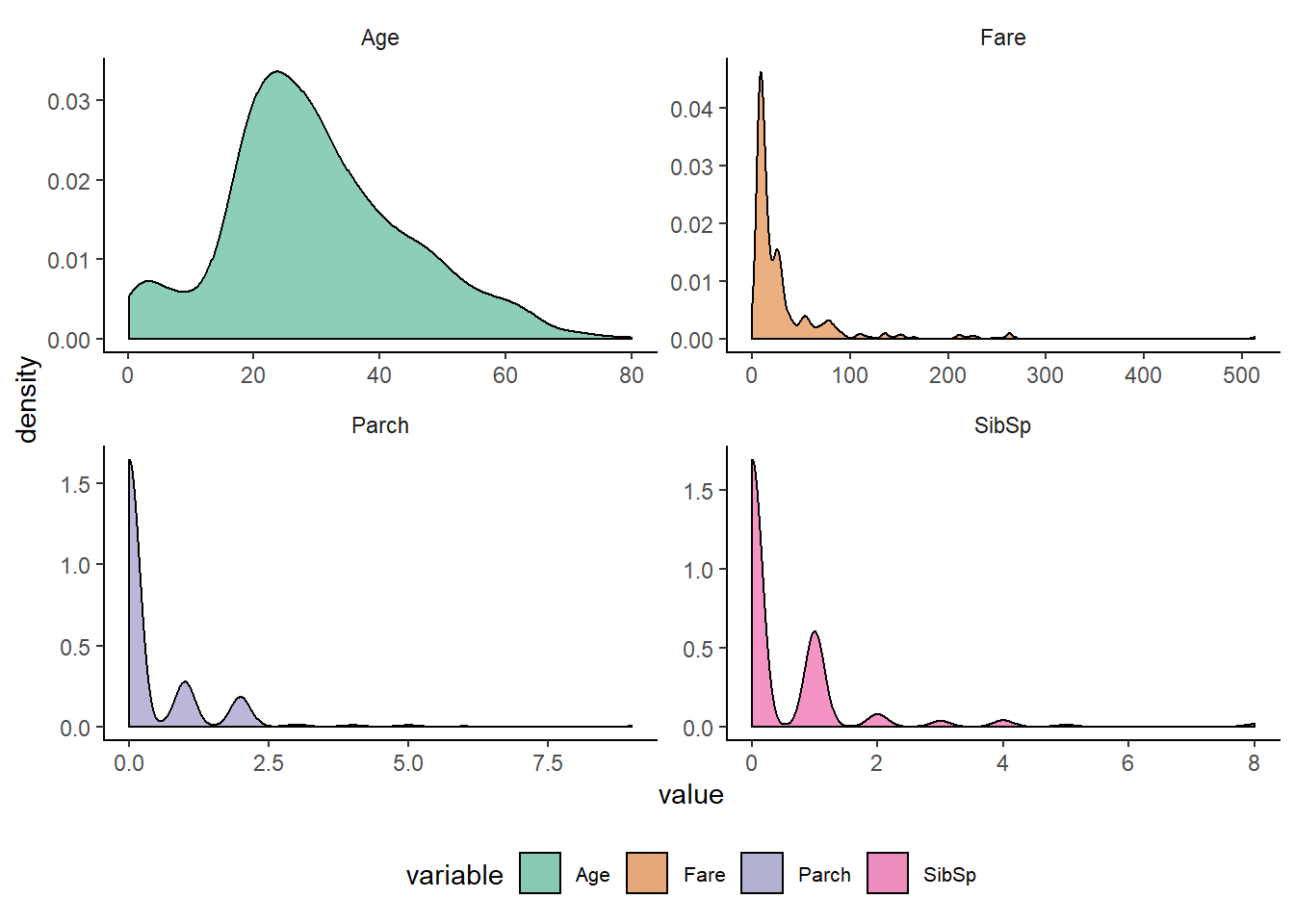
Observation from Density plots :-
- Age has unimodal distribution but has slightly right skewed.
- SibSp, Parch and Fare has multimodal distribution which has again right skewed.
Boxplot :-
It gives a nice summary of one or several numeric variables. The line that divides the box into 2 parts represents the median of the data. The end of the box shows the upper and lower quartiles. The extreme lines shows the highest and lowest value excluding outliers.
num_vars %>%
  gather("variable", "value", 1:4) %>%
  ggplot(aes(y = value, fill = variable))+
  geom_boxplot()+
  mytheme()+
  facet_wrap(~variable, scales = "free")+
  scale_fill_brewer(palette = "Dark2")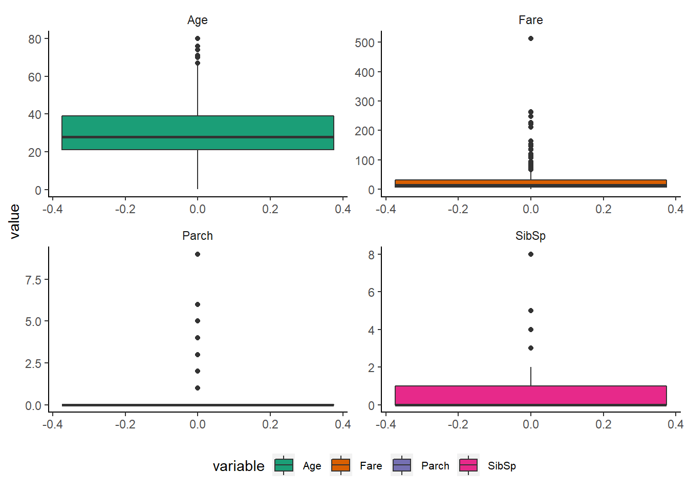
#ggplot(num_vars, aes(x = SibSp,y = Age))+
#  geom_boxplot(fill=I(rgb(0.1,0.2,0.4,0.6)))+
##  geom_text(aes(label = outlier), na.rm = TRUE, hjust = -0.3)+
  #mytheme()
Univariate Analysis of Categorical variable
- Frequencies
- Proportions
- Bar chart for visualization
Selecting categorical variables
cat_vars <- df %>%
  select_if(~!is.numeric(.))
cat_vars %>% head
## # A tibble: 6 x 7
## Survived Pclass Name Sex Ticket Cabin Embarked
## <fct> <fct> <chr> <fct> <chr> <chr> <fct>
## 1 0 3 Braund, Mr. Owen Harris male A/5 21171 <NA> S
## 2 1 1 Cumings, Mrs. John Bradl~ fema~ PC 17599 C85 C
## 3 1 3 Heikkinen, Miss. Laina fema~ STON/O2. ~ <NA> S
## 4 1 1 Futrelle, Mrs. Jacques H~ fema~ 113803 C123 S
## 5 0 3 Allen, Mr. William Henry male 373450 <NA> S
## 6 0 3 Moran, Mr. James male 330877 <NA> QFrequencies and Proportions
Survived
cat_vars %>%
  filter(!is.na(Survived)) %>%
  count(Survived) %>%
  mutate(prop = n/sum(n)) %>%
  arrange(desc(prop))
## # A tibble: 2 x 3
## Survived n prop
## <fct> <int> <dbl>
## 1 0 549 0.616
## 2 1 342 0.384The survival rate among the train set was only 38.38% .
Sex
cat_vars %>%
  count(Sex) %>%
  mutate(prop = n/sum(n)) %>%
  arrange(desc(prop))
## # A tibble: 2 x 3
## Sex n prop
## <fct> <int> <dbl>
## 1 male 843 0.644
## 2 female 466 0.356On ship there were approx 64% were men and 36% were women.
Ticket
cat_vars %>%
  count(Ticket) %>%
  mutate(prop = n/sum(n)) %>%
  arrange(desc(prop))
## # A tibble: 929 x 3
## Ticket n prop
## <chr> <int> <dbl>
## 1 CA. 2343 11 0.00840
## 2 1601 8 0.00611
## 3 CA 2144 8 0.00611
## 4 3101295 7 0.00535
## 5 347077 7 0.00535
## 6 347082 7 0.00535
## 7 PC 17608 7 0.00535
## 8 S.O.C. 14879 7 0.00535
## 9 113781 6 0.00458
## 10 19950 6 0.00458
## # ... with 919 more rowsCabin
cat_vars %>%
  count(Cabin) %>%
  mutate(prop = n/sum(n)) %>%
  arrange(desc(prop)) %>%
  head
## # A tibble: 6 x 3
## Cabin n prop
## <chr> <int> <dbl>
## 1 <NA> 1014 0.775
## 2 C23 C25 C27 6 0.00458
## 3 B57 B59 B63 B66 5 0.00382
## 4 G6 5 0.00382
## 5 B96 B98 4 0.00306
## 6 C22 C26 4 0.00306- Around 77% values in Cabin column were missing so its better to drop this feature from our analysis.
Embarked
cat_vars %>%
  count(Embarked) %>%
  mutate(prop = n/sum(n)) %>%
  arrange(desc(prop))
## # A tibble: 4 x 3
## Embarked n prop
## <fct> <int> <dbl>
## 1 S 914 0.698
## 2 C 270 0.206
## 3 Q 123 0.0940
## 4 <NA> 2 0.00153- Around 70% of passenger were embarked from Southampton and 20 % from Cherbourg and remaining from Queenstown.
Barcharts for visualization
cat_vars %>%
  subset(!is.na(Survived)) %>%
  select(Pclass, Sex,Embarked, Survived) %>%
  gather("variable", "value", 1:4) %>%
  ggplot(aes(y= variable, x = value, fill = variable))+
  geom_col()+
  mytheme()+
  facet_wrap(~variable, scales = "free")+
  scale_fill_brewer(palette = "Dark2")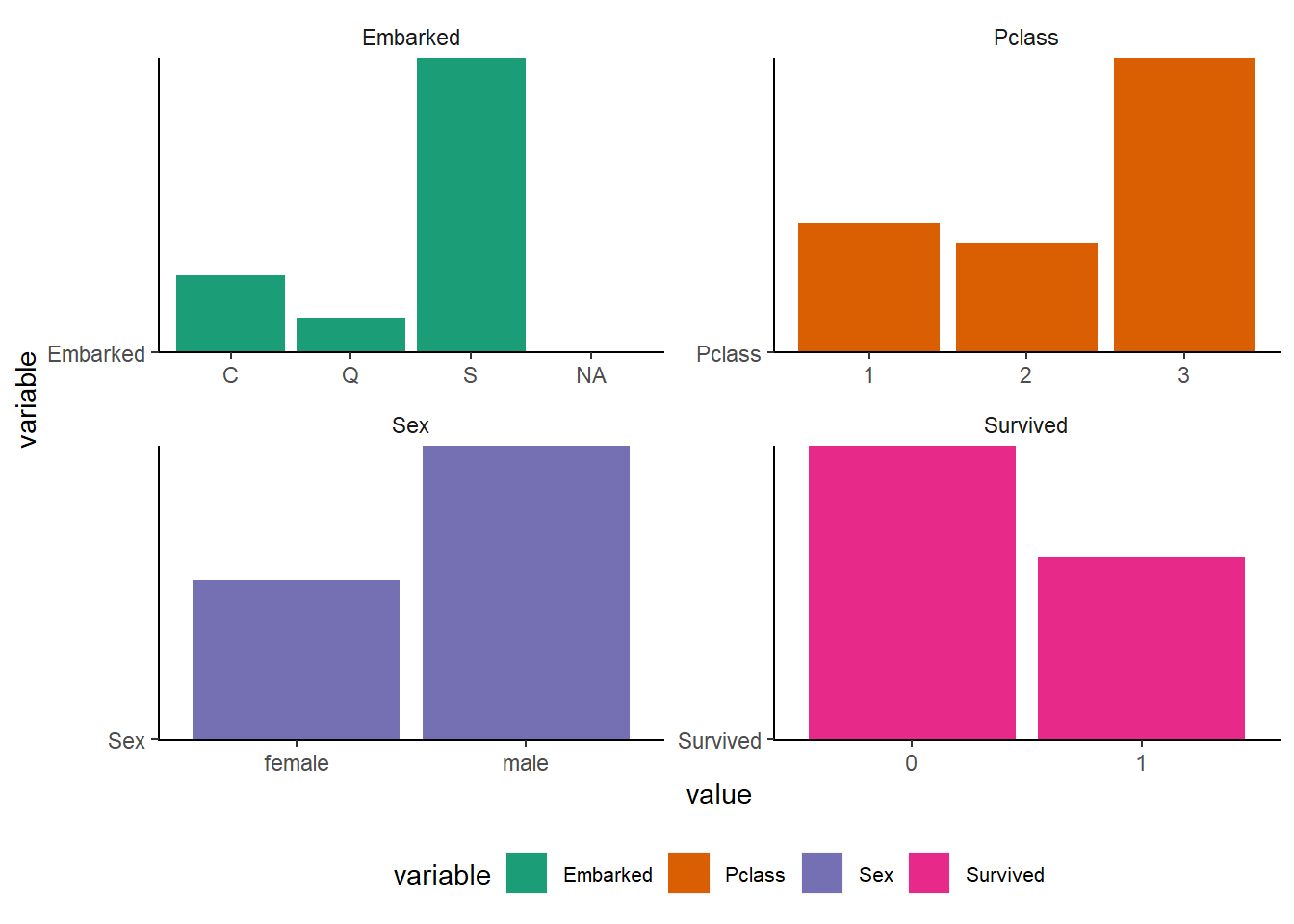
Bi-variate Analysis
Here we look for relationship between two variables.There are 3 kinds of combination for bivariate analysis for continuos and categorical variable.
Continuos-Continuos
- Correlation :- It find the strength of relationship (-1 Perfect Negative Correlation, 1 perfect Positive Correlation, 0 No Correlation )
- Scatter plot :- It shows relationship between 2 variable.(linear or nonlinear)
Categorical- Categorical
- Two way table :- Show the relationship by creating a two-way table of count and count%
- Stacked Column Chart:- A visual form of Two-way table
- Chi-Square test:-
Categorical-Continuos
- Visualization methods
- Z-test/T-test
- ANOVA
Ok lets start Bivariate Analysis with continuos-continuos variable.
Correlation :-
library(corrplot)
df %>%
  select(-Name, -Cabin, -Ticket) %>%
  mutate(Sex = fct_recode(Sex, "0" = "male", "1" ="female")) %>%
  mutate(Survived = as.integer(Survived),
         Sex = as.integer(Sex),
         Pclass = as.integer(Pclass),
         Embarked = as.integer(Embarked)) %>%
  cor(use = "complete.obs") %>%
  corrplot(type ="lower", diag = FALSE)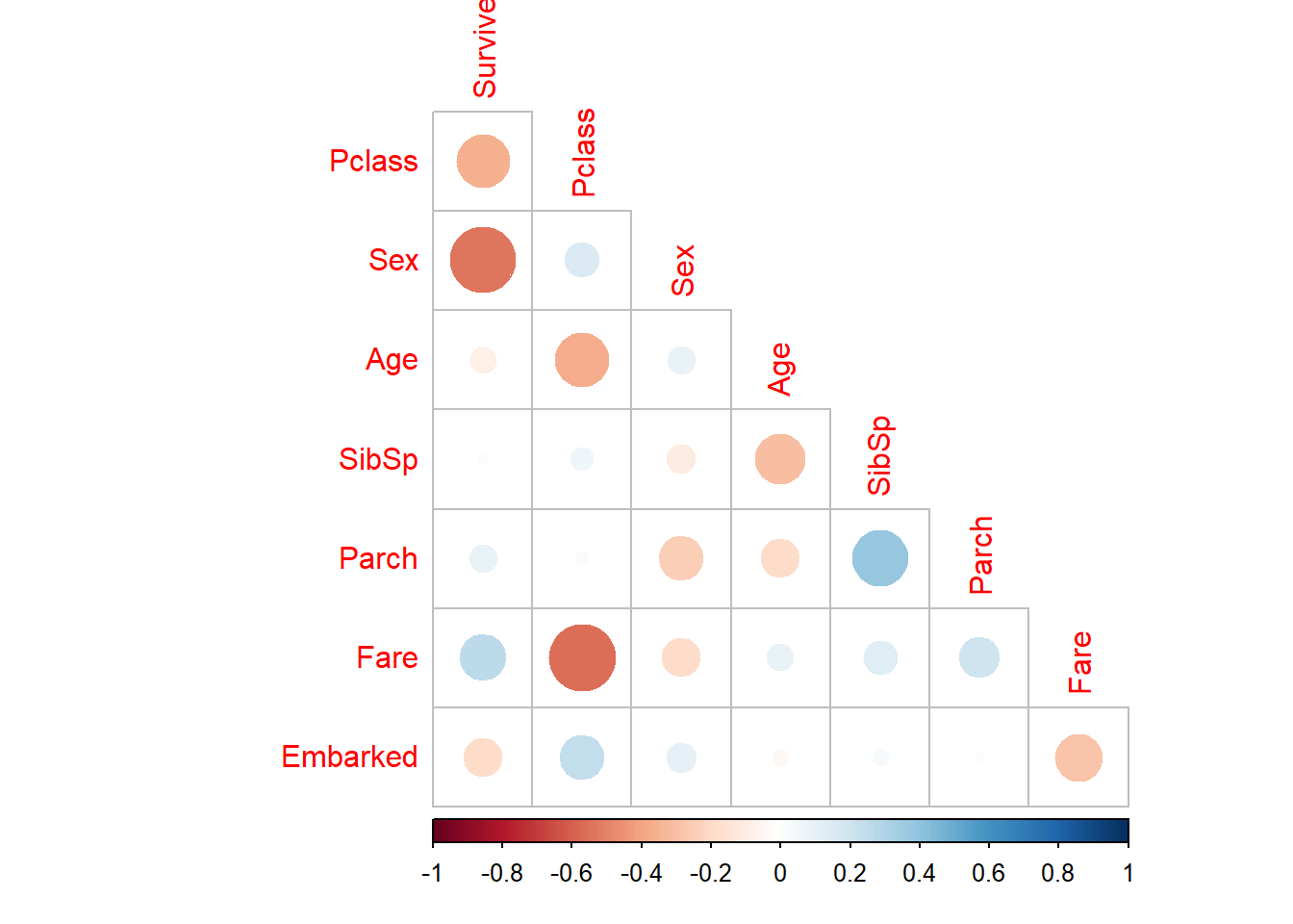
Observations:-
- Survived is correlate most to Sex, and then to Pclass.
- Fare and Embarked might play a secondary role; the other features are pretty weak.
- Fare and Pclass are strongly related (1st-class cabins will be more expensive)
- A correlation of SibSp and Parch makes intuitive sense (both indicate family size)
- Pclass and Age seem related (richer people are on average older? not inconceivable)
From above overview plot we would like to study in more details following relationships wrt to target variable under multivariate analysis :-
- Pclass vs Fare
- Pclass vs Age
- Pclass vs Embarked
- Sex vs Parch
- Age vs Sibsp
- Sibsp Vs Parch
- Fare vs Embarked
Categorical - Categorical
1.Two way table
cat_vars %>% head()## # A tibble: 6 x 7
## Survived Pclass Name Sex Ticket Cabin Embarked
## <fct> <fct> <chr> <fct> <chr> <chr> <fct>
## 1 0 3 Braund, Mr. Owen Harris male A/5 21171 <NA> S
## 2 1 1 Cumings, Mrs. John Bradl~ fema~ PC 17599 C85 C
## 3 1 3 Heikkinen, Miss. Laina fema~ STON/O2. ~ <NA> S
## 4 1 1 Futrelle, Mrs. Jacques H~ fema~ 113803 C123 S
## 5 0 3 Allen, Mr. William Henry male 373450 <NA> S
## 6 0 3 Moran, Mr. James male 330877 <NA> Qtable(cat_vars$Survived, cat_vars$Pclass)##
## 1 2 3
## 0 80 97 372
## 1 136 87 119mytable <- table(cat_vars$Survived, cat_vars$Pclass)
prop.table(mytable,2)##
## 1 2 3
## 0 0.3703704 0.5271739 0.7576375
## 1 0.6296296 0.4728261 0.2423625prop.table(ftable(table(cat_vars$Pclass,cat_vars$Sex,cat_vars$Survived)),1)*100## 0 1
##
## 1 female 3.191489 96.808511
## male 63.114754 36.885246
## 2 female 7.894737 92.105263
## male 84.259259 15.740741
## 3 female 50.000000 50.000000
## male 86.455331 13.544669xtabs(~Survived+Pclass+Sex, data = cat_vars)## , , Sex = female
##
## Pclass
## Survived 1 2 3
## 0 3 6 72
## 1 91 70 72
##
## , , Sex = male
##
## Pclass
## Survived 1 2 3
## 0 77 91 300
## 1 45 17 472.Stacked Column Chart
- Sex Vs Survived
- Pclass Vs Survived
- Parch Vs Survived
- SibSp Vs Survived
- Embarked Vs Survived
#fill <- c("#778899", "#D3D3D3")
p3 <- ggplot(subset(df, !is.na(Survived)), aes(x = Sex, fill = Survived))+
  geom_bar(stat = "count", position = "fill")+
  mytheme()+
  labs(title = "Sex")+
  scale_fill_brewer(palette = "Dark2")

p4 <- ggplot(subset(df, !is.na(Survived)), aes(x = Pclass, fill = Survived))+
  geom_bar(stat = "count", position = "fill")+
  mytheme()+
  theme(legend.position = "none")+
  labs(title = "Pclass")+
  scale_fill_brewer(palette = "Dark2")

p5 <- ggplot(subset(df, !is.na(Survived)), aes(x = Parch,fill = Survived))+
  geom_bar(stat = "count", position = "fill")+
  mytheme()+
  theme(legend.position = "none")+
  labs(title = "Parch")+
  scale_fill_brewer(palette = "Dark2")

p6 <- ggplot(subset(df, !is.na(Survived)), aes(x = SibSp, fill = Survived))+
  geom_bar(stat = "count", position = "fill")+
  mytheme()+
  theme(legend.position = "none")+
  labs(title = "Sibsp")+
  scale_fill_brewer(palette = "Dark2")

p7 <- ggplot(subset(df, !is.na(Survived)), aes(x = Embarked, fill = Survived))+
  geom_bar(stat = "count", position = "fill")+
  mytheme()+
  labs(title = "Embarked")+
  scale_fill_brewer(palette = "Dark2")
gridExtra::grid.arrange(p3,p4,p5,p6,p7, ncol = 2)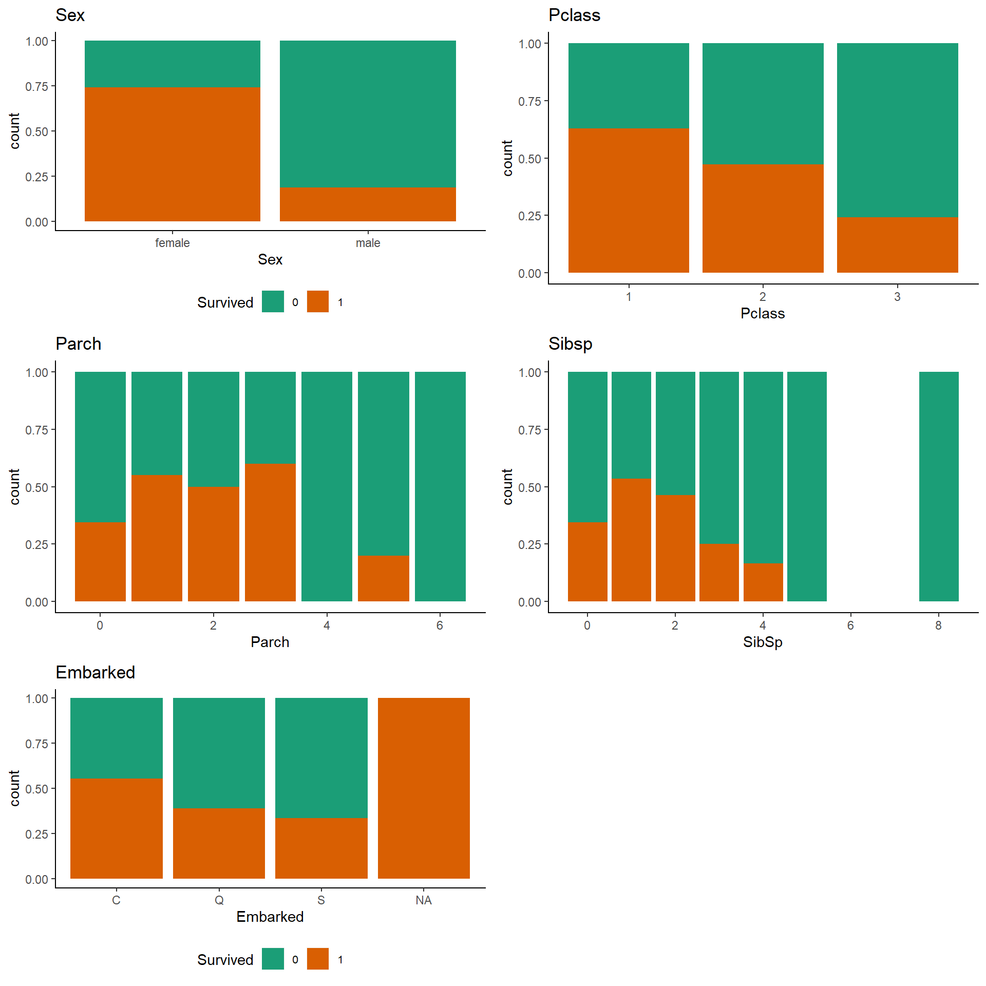
Observations :-
Pclass
There’s a clear trend that being a 1st class passenger gives you better chances of survival.
SibSP/Parch
Having 1-3 siblings/spouses/parents/children on board (SibSp = 1-2, Parch = 1-3) suggests proportionally better survival numbers than being alone (SibSp + Parch = 0) or having a large family travelling with you.
Embarked
Well, that does look more interesting than expected. Embarking at “C” resulted in a higher survival rate than embarking at “S”. There might be a correlation with other variables, here though
Categorical- Continuos
- Age Vs Survived
- Fare Vs Survived
#color <- c("#778899", "#D3D3D3")
p1 <- ggplot(subset(df, !is.na(Survived)), aes(x = Fare, color = Survived))+
  geom_freqpoly(binwidth =0.05)+
  scale_x_log10() +
  guides(fill = FALSE)+
  theme(legend.position = "none")+
  mytheme()+
  labs(title = "Fare")+
  scale_color_brewer(palette = "Dark2")

p2 <-  ggplot(subset(df, !is.na(Survived)), aes(x = Age, color = Survived))+
  geom_freqpoly(binwidth =1)+
  guides(fill = FALSE)+
  theme(legend.position = "none")+
  mytheme()+
  labs(title = "Age")+
  scale_color_brewer(palette = "Dark2")

gridExtra::grid.arrange(p1,p2, ncol=2)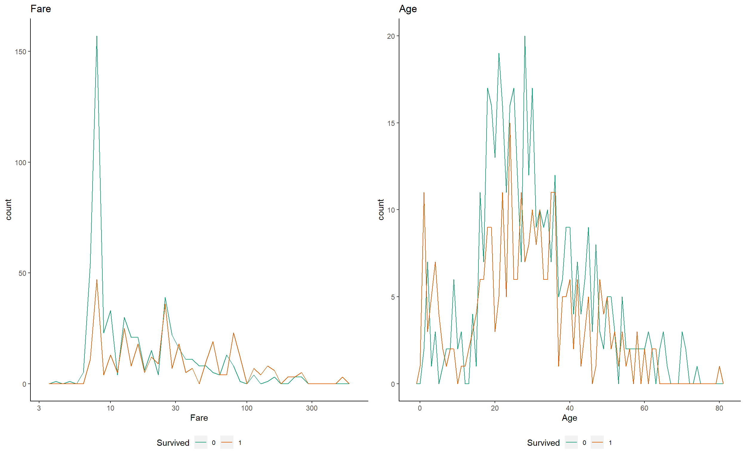
Observations :-
Age
- Fewer young adults have survived (ages 18 - 30-ish) whereas children younger than 10-ish had better survival rate .
- The highest ages are well consistent with the overall distribution
Fare
- This is case where a linear scaling isn’t of much help because there is a smaller number of more extreme numbers. A natural choice in this case is to use a logarithmic axis.
- The plot tells us that the survival chances were much lower for the cheaper cabins.
- One would assume that those cheap cabins were mostly located deeper inside the ship
Z-test :-
Lets say we want to check the significance of a variable Pclass. Let’s assume that upper class has better chances of survival than its population.
To verify this we will use z-test.
H0 :- There is no significant difference between chances of survival of lower and upper class.
HA :- There is better chances of survival of upper class.
train$Survived <- as.numeric(train$Survived)
new_train <-  subset(train, train$Pclass == 1)
#function for z test
z.test2 = function(a, b, n){
sample_mean = mean(a)
pop_mean = mean(b)
c = nrow(n)
var_b = var(b)
zeta = (sample_mean - pop_mean) / (sqrt(var_b/c))
return(zeta)
}
z.test2(new_train$Survived, train$Survived, new_train)## [1] 7.423828If |z| < 1.96 then difference is not significant at 5%. and if |z|>= 1.96 then difference is significant at 5%.
Our Z value comes out to be 7.42 which affirms our suggestion that upper class has better chances of survival than its population.
Chi Square Test :-
chisq.test(train$Survived, train$Sex)##
## Pearson's Chi-squared test with Yates' continuity correction
##
## data: train$Survived and train$Sex
## X-squared = 260.72, df = 1, p-value < 2.2e-16summary(table(train$Survived, train$Pclass))## Number of cases in table: 891
## Number of factors: 2
## Test for independence of all factors:
## Chisq = 102.89, df = 2, p-value = 4.549e-23Since -P-value is less than 0.05 we can infer that Sex and Pclass are highly significant variables and must be included in the modelling.
Anova:-
- Anova simply check if atleast one of two or more groups have statistically differnt means.
- We use ANOVA test to understand the correlation between atleast one categorical variable with two or more factor levels and continuos response variable.
- Anova is measured using a statistic known as F-ratio. It is defined as the ratio of mean square between groups to the mean square with in group.
- Anova is used in Machine learning modelling to identify whether a categorical variable is relevant to a continuos variable. Also whether a treatment is effective to model or not.
Pclass vs Fare
#fill <- c("#778899", "#D3D3D3")
ggplot(subset(df, !is.na(Survived)), aes(Pclass, Fare, fill = Survived))+
  geom_boxplot()+
  scale_y_log10()+
  mytheme()+
  scale_fill_brewer(palette = "Dark2")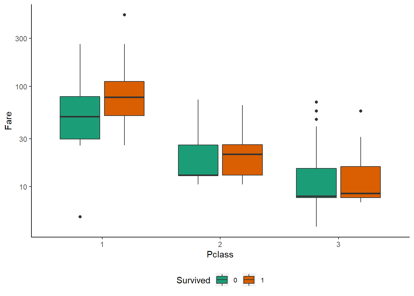
Observations :-
The different Pclass categories are clustered around different average levels of Fare. This is not very surprising, as 1st class tickets are usually more expensive than 3rd class ones.
In 2nd Pclass, and especially in 1st, the median Fare for the Survived == 1 passengers is notably higher than for those who died. This suggests that there is a sub-division into more/less expensive cabins (i.e. closer/further from the life boats) even within each Pclass.
It’s certainly worth to have a closer look at the Fare distributions depending on Pclass. In order to contrast similar plots for different factor feature levels ggplot2 offers the facet mechanism. Adding facets to a plot allows us to separate it along one or two factor variables. Naturally, this visualisation approach works best for relatively small numbers of factor levels.
#fill <- c("#778899", "#D3D3D3", "#ff6347")
df %>%
  subset(!is.na(Survived)) %>%

  ggplot(aes(Fare, fill=Pclass)) +

  geom_density(alpha = 0.5) +

  scale_x_log10() +

  facet_wrap(~ Survived, ncol = 1)+
  mytheme()+
  scale_fill_brewer(palette = "Dark2")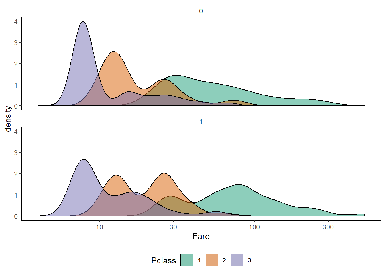
Observations :-
- There is a suprisingly broad distribution between the 1st class passenger fares
- There’s an interesting bimodality in the 2nd class cabins and a long tail in the 3rd class ones
- For each class there is strong evidence that the cheaper cabins were worse for survival. A similar effect can be seen in a boxplot.
Pclass vs Embarked
#fill <- c("#778899", "#D3D3D3", "#ff6347")
df %>%
  subset(!is.na(Survived)) %>%
  filter(Embarked %in% c("S","C","Q")) %>%
  ggplot() +
  geom_bar(aes(Embarked, fill = Pclass), position = "dodge") +
  facet_grid(~ Survived)+
  scale_fill_brewer(palette = "Dark2")+
  mytheme()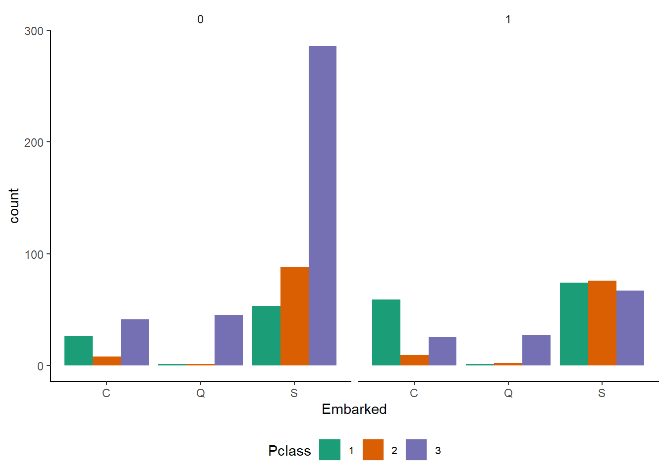
Observations :-
- Embarked Q contains most exclusively 3rd class passengers.
- The survival chances for 1st class passengers are better for every port. In contrast, the chances for the 2nd class passengers were relatively worse for Embarked == S whereas the frequencies for Embarked == C look comparable.
- 3rd class passengers had bad chances everywhere, but the relative difference for Embarked == S looks particularly strong.
Pclass vs Age
#fill <- c("#778899",  "#ff6347")
df %>%
  subset(!is.na(Survived)) %>%
  filter(Embarked %in% c("S","C","Q")) %>%
  ggplot(mapping = aes(Age, Fare, color = Survived, shape = Sex)) +
  geom_point() +
  scale_y_log10() +
  facet_grid(Pclass ~ Embarked)+
  theme_minimal()+
  scale_color_brewer(palette = "Dark2")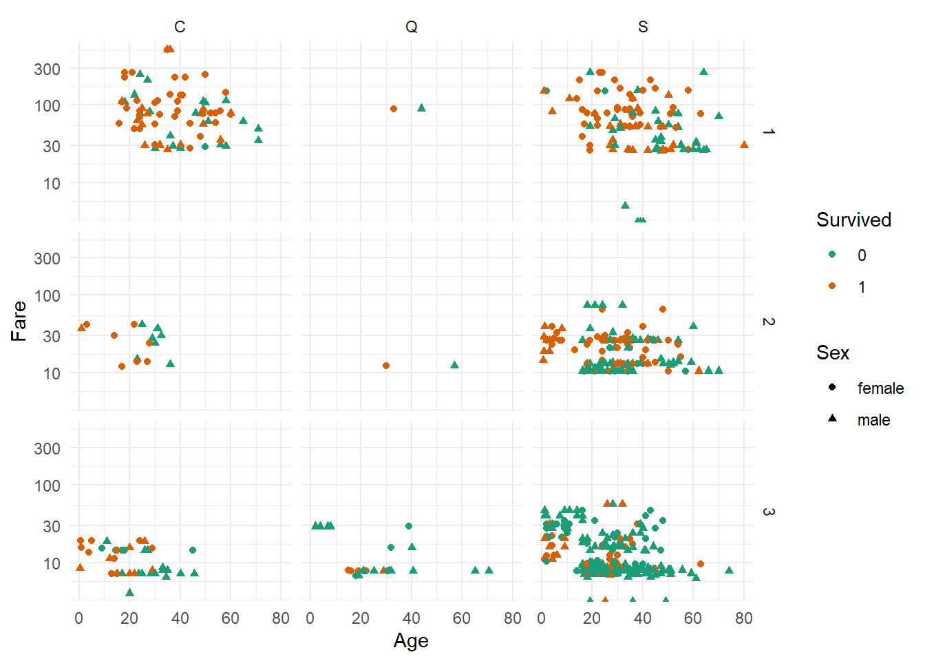
Observations :-
1. Pclass == 1 passengers seem indeed on average older than those in 3rd (and maybe 2nd) class. Not many children seemed to have travelled 1st class.
2. Most Pclass == 2 children appear to have survived, regardless of Sex.
3. More men than women seem to have travelled 3rd Pclass, whereas for 1st Pclass the ratio looks comparable. Note, that those are only the ones for which we know the Age, which might introduce a systematic bias.
Age vs Sex This was not in our original list but multi-facet plot above prompt us to examine the interplay between Age and sex.
#fill <- c("#778899", "#ff6347")
ggplot(subset(df,!is.na(Survived)), aes(x=Age)) +

  geom_density(aes(fill = Survived), alpha = 0.5) +

  facet_wrap(~Sex)+
  mytheme()+
  scale_fill_brewer(palette = "Dark2")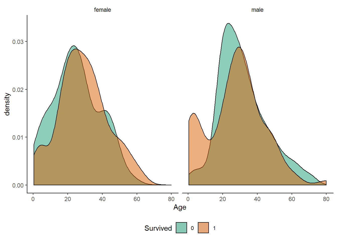
observations :-
1. Younger boys had a notable survival advantage over male teenagers, whereas the same was not true for girls to nearly the same extent.
2. Most women over 60 survived, whereas for men the high-Age tail of the distribution falls slower.
3. Note that those are normalised densities, not histogrammed numbers. Also, remember that Age contains many missing values.
Pclass vs Sex
mosaicplot(table(train$Survived,train$Sex, train$Pclass ),
           main = "Survival by Pclass and Sex" , shade = TRUE)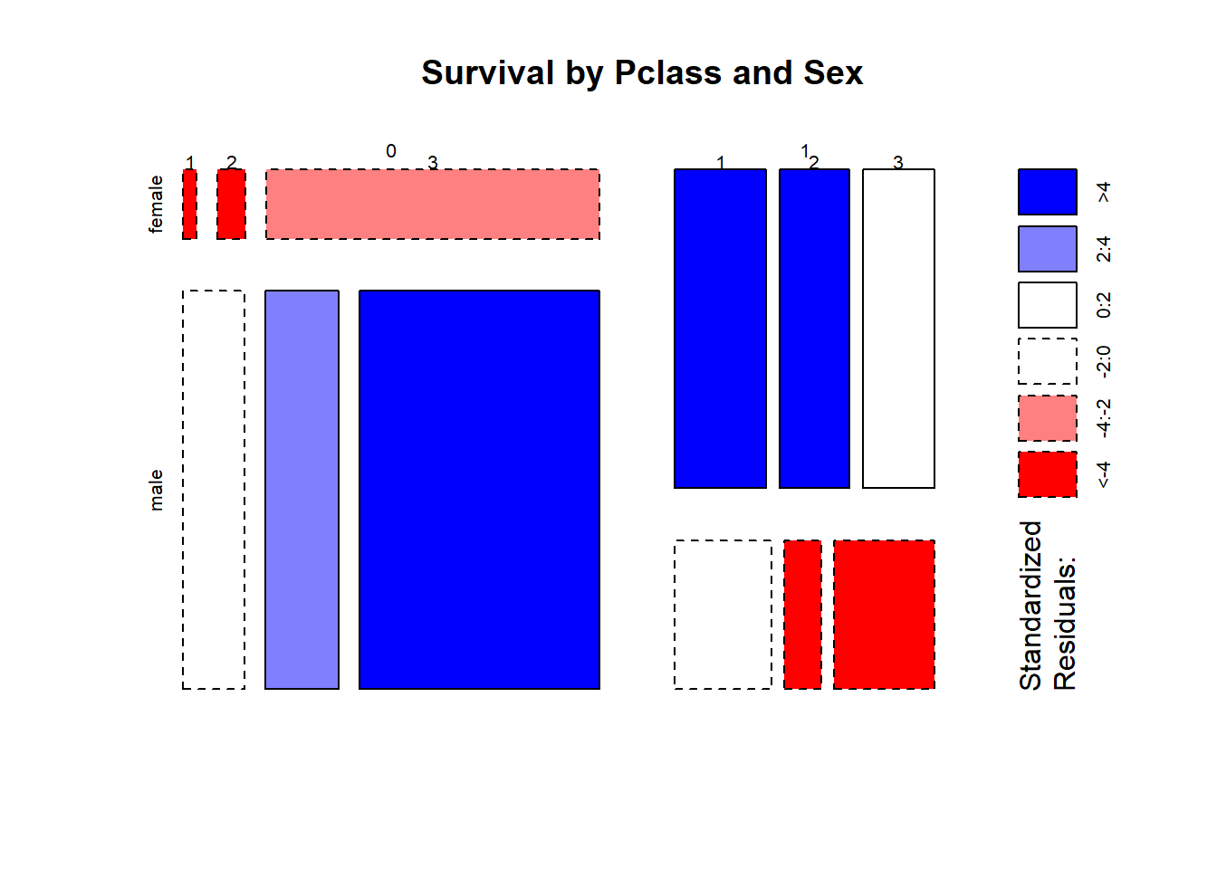
Observations :-
- Almost all females that died were 3rd Plass passengers.
- For the males, being in 3rd Pclass resulted in a significant disadvantage regarding their Survived status.
Parch vs SibSp
train %>%
ggplot(aes(Parch, SibSp, color = as.factor(Survived))) +
geom_count()+
mytheme()+
scale_color_brewer(type = "seq",palette = "Dark2")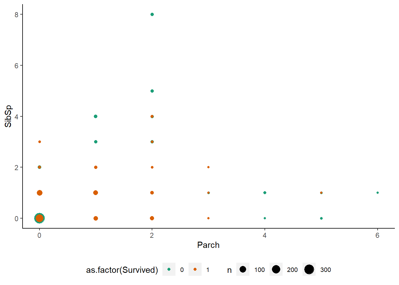
Observations :-
- A large number of passengers were travelling alone.
- Passengers with the largest number of parents/children had relatively few siblings on board.
- Survival was better for smaller families, but not for passengers travelling alone.
Parch vs Sex
#fill <- c("#778899", "#D3D3D3")
train %>%

  ggplot() +

  geom_bar(aes(Parch, fill = Sex), position = "dodge") +

  scale_y_log10()+
  mytheme()+
 scale_fill_brewer(palette = "Dark2")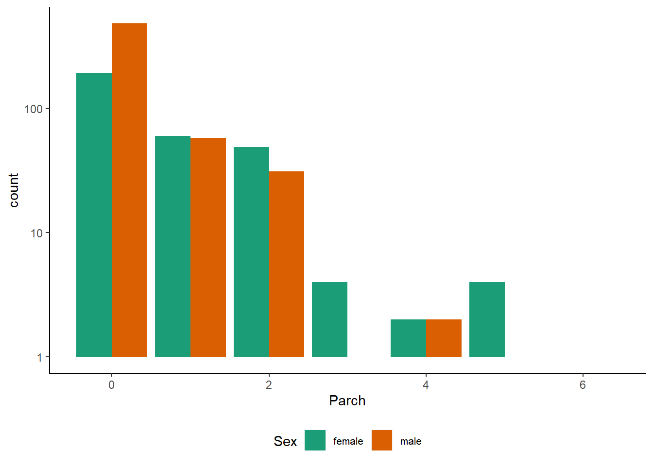
Observations :-
Many more men travelled without parents or children than women did. The difference might look small here but that’s because of the logarithmic y-axis.
The log axis helps us to examine the less frequent Parch levels in more detail: Parch == 2,3 still look comparable. Beyond that, it seems that women were somewhat more likely to travel with more relatives. However, beware of small numbers
train %>%
  group_by(Parch,Sex) %>%
  count
## # A tibble: 13 x 3
## # Groups: Parch, Sex [13]
## Parch Sex n
## <dbl> <chr> <int>
## 1 0 female 194
## 2 0 male 484
## 3 1 female 60
## 4 1 male 58
## 5 2 female 49
## 6 2 male 31
## 7 3 female 4
## 8 3 male 1
## 9 4 female 2
## 10 4 male 2
## 11 5 female 4
## 12 5 male 1
## 13 6 female 1Age Vs SibSp
train %>%
mutate(SibSp = factor(SibSp)) %>%
ggplot(aes(x=Age, color = SibSp)) +
geom_density(size = 1.0)+
mytheme()+
scale_color_brewer(palette = "Dark2")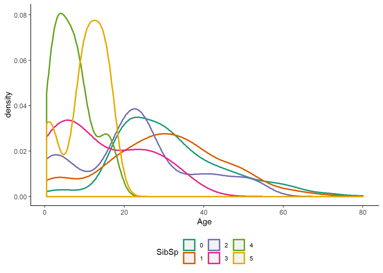 Observations :-
1. The highest SibSp values (4 and 5) are indeed associated with a narrower distribution peaking at a lower Age. Most likely groups of children from large families.
Some times good graphical animation helpful in telling the data story without saying words. Also to impress the your audience. gganimation package comes very handy here.
To learn more about animation using gganimate package click here
Here i am showing some demo examples.
train %>%
  mutate(Survived = as.numeric(Survived)) %>%
  ggplot( aes(Parch, SibSp ,fill = Survived))+
  geom_tile(colour  = "white")+
  facet_grid(Pclass~Sex)+
  scale_fill_gradient(low ="tomato", high = "darkgreen")+
  labs(x="",
       y="",
       title = 'Fare: {frame_time}',
       subtitle="Kaggle data",
       fill="Close")+
  transition_time(Fare)+
  ease_aes('linear', interval = 0.00001)+
  mytheme()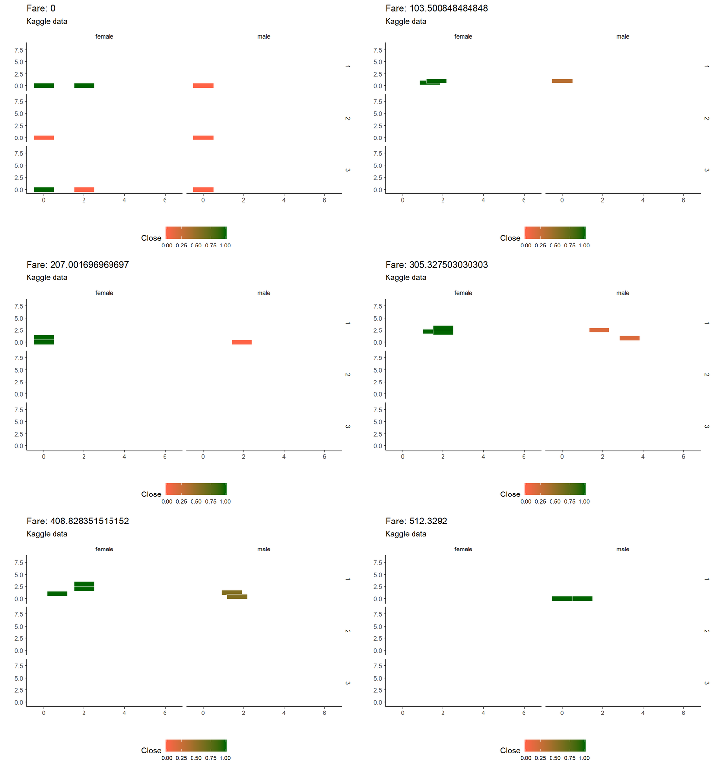
train %>%
  ggplot(aes(x = Age, y = Fare))+
  geom_point(aes(color = Survived), size = 2)+
  transition_states(Sex,
                    transition_length = 1,
                    state_length = 1)+
  mytheme()+
  enter_fade() +
  labs(x="Age",
       y="Fare",
       title = "{closest_state}",
       subtitle="Kaggle data",
       fill="Close")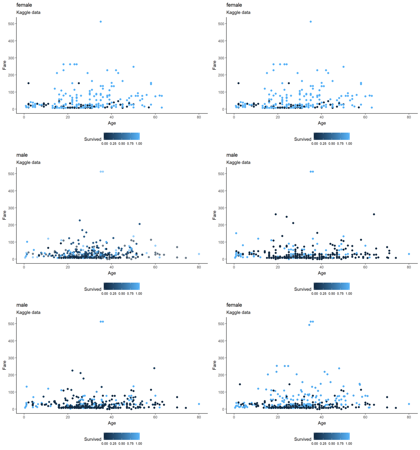
Missing Values Treatment
Types of Missing Values :-
1.Missing Completely at random
2.Missing at random
3.Missing that depends on unobserved predictors
4.Missing that depends on the missing value itself
1. Missing Completely at random :-
A case when the probability of missing variable is same for all observations.
2. Missing at random :-
A case when variable is missing at random and missing ratio varies for different values / level of other input variables. For example: We are collecting data for age and female has higher missing value compare to male.
3. Missing that depends on unobserved predictors :-
A case when the missing values are not random and are related to the unobserved input variable.
4. Missing that depends on the missing value itself :-
A case when the probability of missing value is directly correlated with missing value itself. For example: People with higher or lower income are likely to provide non-response to their earning.
Treatment of Missing Values
Deletion :-
1.1 List wise deletion:- Delete complete observation when there is any of the variable missing.
1.2 Pair wise deletion:- Perform analysis with all cases in which the variables of interest are present.Imputaton :-
2.1 Generalized Imputation :-
Calculate the mean or median for all non missing values of that variable then replace missing value with mean or median.
2.2 Similar Case Imputation :-
Calculate mean/median/mode based on some other variable and replace based upon it. For example :- Replacing value of age based on gender.
Mean :- Replace the missing data for a given attribute (quantitative) by mean when data is not skewed.
Median :- Replace the missning data for a given attribute(quantitative) by median when data is skewed.
Mode :- Replace the missing data for a given attribute( Qualitative) by mode.
- Prediction Model :-
Create a predictive model to estimate values that will substitute the missing data.
- KNN Imputation :-
The missing values of an attribute are imputed using the given number of attributes that are most similar to the attribute whose values are missing. The similarity of two attributes is determined using a distance function.
Lets check for the missing values in the columns
df %>%
    map_df(function(x) sum(is.na(x)))
## # A tibble: 1 x 11
## Survived Pclass Name Sex Age SibSp Parch Ticket Fare Cabin Embarked
## <int> <int> <int> <int> <int> <int> <int> <int> <int> <int> <int>
## 1 418 0 0 0 263 0 0 0 1 1014 2#df %>% summarise_all(list(~sum(is.na(.)))) Following are the observations from the above table:-
1.The 418 NA in survived column are the observations in test dataset.
2.Age has 263 missing values.
3.Cabin has significant number of missing values. i.e. 1014.
4.Also Embarked Fare has 2 and 1 missing values respectively.
Missing Value Imputation
Age
For imputing missing value in age we will use mice package.
# Make variables factors into factors
factor_vars <- c('Pclass','Sex','Embarked')

df[factor_vars] <- lapply(df[factor_vars], function(x) as.factor(x))

# Set a random seed
set.seed(129)

# Perform mice imputation, excluding certain less-than-useful variables:
mice_mod <- mice(df[, !names(df) %in% c('Name','Ticket','Cabin','Survived')], method='rf')
##
## iter imp variable
## 1 1 Age Fare Embarked
## 1 2 Age Fare Embarked
## 1 3 Age Fare Embarked
## 1 4 Age Fare Embarked
## 1 5 Age Fare Embarked
## 2 1 Age Fare Embarked
## 2 2 Age Fare Embarked
## 2 3 Age Fare Embarked
## 2 4 Age Fare Embarked
## 2 5 Age Fare Embarked
## 3 1 Age Fare Embarked
## 3 2 Age Fare Embarked
## 3 3 Age Fare Embarked
## 3 4 Age Fare Embarked
## 3 5 Age Fare Embarked
## 4 1 Age Fare Embarked
## 4 2 Age Fare Embarked
## 4 3 Age Fare Embarked
## 4 4 Age Fare Embarked
## 4 5 Age Fare Embarked
## 5 1 Age Fare Embarked
## 5 2 Age Fare Embarked
## 5 3 Age Fare Embarked
## 5 4 Age Fare Embarked
## 5 5 Age Fare Embarked# Save the complete output
mice_output <- complete(mice_mod)summary(df)## Survived Pclass Name Sex Age
## 0 :549 1:323 Length:1309 female:466 Min. : 0.17
## 1 :342 2:277 Class :character male :843 1st Qu.:21.00
## NA's:418 3:709 Mode :character Median :28.00
## Mean :29.88
## 3rd Qu.:39.00
## Max. :80.00
## NA's :263
## SibSp Parch Ticket Fare
## Min. :0.0000 Min. :0.000 Length:1309 Min. : 0.000
## 1st Qu.:0.0000 1st Qu.:0.000 Class :character 1st Qu.: 7.896
## Median :0.0000 Median :0.000 Mode :character Median : 14.454
## Mean :0.4989 Mean :0.385 Mean : 33.295
## 3rd Qu.:1.0000 3rd Qu.:0.000 3rd Qu.: 31.275
## Max. :8.0000 Max. :9.000 Max. :512.329
## NA's :1
## Cabin Embarked
## Length:1309 C :270
## Class :character Q :123
## Mode :character S :914
## NA's: 2
##
##
## summary(mice_output)## Pclass Sex Age SibSp Parch
## 1:323 female:466 Min. : 0.17 Min. :0.0000 Min. :0.000
## 2:277 male :843 1st Qu.:21.00 1st Qu.:0.0000 1st Qu.:0.000
## 3:709 Median :28.00 Median :0.0000 Median :0.000
## Mean :29.55 Mean :0.4989 Mean :0.385
## 3rd Qu.:38.00 3rd Qu.:1.0000 3rd Qu.:0.000
## Max. :80.00 Max. :8.0000 Max. :9.000
## Fare Embarked
## Min. : 0.000 C:270
## 1st Qu.: 7.896 Q:124
## Median : 14.454 S:915
## Mean : 33.281
## 3rd Qu.: 31.275
## Max. :512.329summary(df$Age)## Min. 1st Qu. Median Mean 3rd Qu. Max. NA's
## 0.17 21.00 28.00 29.88 39.00 80.00 263# Plot age distributions
par(mfrow=c(1,2))
hist(df$Age, freq=F, main='Age: Original Data',
col='#D95F02', ylim=c(0,0.04))
hist(mice_output$Age, freq=F, main='Age: MICE Output',
col="#1B9E77", ylim=c(0,0.04))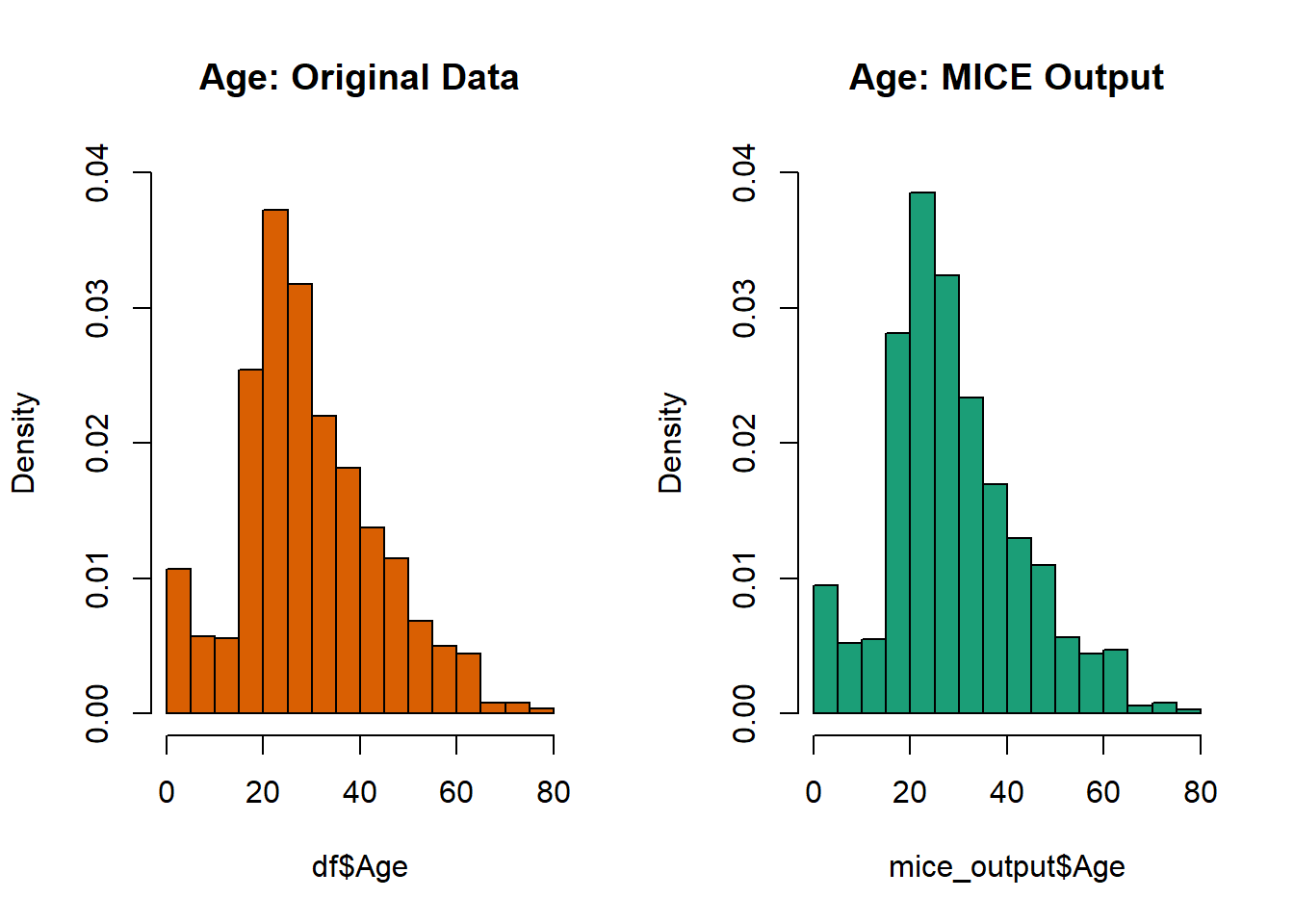
# Replace Age variable from the mice model.
df$Age <- mice_output$Age

# Show new number of missing Age values
sum(is.na(df$Age))
## [1] 0Cabin
df %>% filter(is.na(Cabin))## # A tibble: 1,014 x 11
## Survived Pclass Name Sex Age SibSp Parch Ticket Fare Cabin
## <fct> <fct> <chr> <fct> <dbl> <dbl> <dbl> <chr> <dbl> <chr>
## 1 0 3 Brau~ male 22 1 0 A/5 2~ 7.25 <NA>
## 2 1 3 Heik~ fema~ 26 0 0 STON/~ 7.92 <NA>
## 3 0 3 Alle~ male 35 0 0 373450 8.05 <NA>
## 4 0 3 Mora~ male 19 0 0 330877 8.46 <NA>
## 5 0 3 Pals~ male 2 3 1 349909 21.1 <NA>
## 6 1 3 John~ fema~ 27 0 2 347742 11.1 <NA>
## 7 1 2 Nass~ fema~ 14 1 0 237736 30.1 <NA>
## 8 0 3 Saun~ male 20 0 0 A/5. ~ 8.05 <NA>
## 9 0 3 Ande~ male 39 1 5 347082 31.3 <NA>
## 10 0 3 Vest~ fema~ 14 0 0 350406 7.85 <NA>
## # ... with 1,004 more rows, and 1 more variable: Embarked <fct>Cabin has lot of missing value so its better to drop this variable.
df$Cabin <- NULLEmbarked
df %>% filter(is.na(Embarked))## # A tibble: 2 x 10
## Survived Pclass Name Sex Age SibSp Parch Ticket Fare Embarked
## <fct> <fct> <chr> <fct> <dbl> <dbl> <dbl> <chr> <dbl> <fct>
## 1 1 1 Icard, Mis~ fema~ 38 0 0 113572 80 <NA>
## 2 1 1 Stone, Mrs~ fema~ 62 0 0 113572 80 <NA>So here there are two females one adult and other Senior for whom Embarked feature has missing values.Both the females are from first class with same fare ($80) and had stayed in same cabin (B28). This makes high chance of both embarked from the same port.
if we look the frequency of ports of embarkation of first class passenger.
df %>% filter(Pclass==1) %>% count(Embarked)## # A tibble: 4 x 2
## Embarked n
## <fct> <int>
## 1 C 141
## 2 Q 3
## 3 S 177
## 4 <NA> 2The Southampton port is the most frequent port of embarkation with 177 ports and it is followed by the Cherbourg port with 141. But still we cannot decide to impute two missing values by the most frequent port of embarkation which is the Southampton port.
ggplot(filter(df, is.na(Embarked)==FALSE & Embarked!='' & Pclass==1),
       aes(Embarked, Fare)) +
  geom_boxplot(aes( fill= Embarked)) +
  geom_hline(aes(yintercept=80), colour='red', linetype='dashed', size=2) +
  ggtitle("Fare distribution of first class passengers") +
  mytheme() +
  theme(plot.title = element_text(hjust = 0.5))+
  scale_fill_brewer(palette = "Dark2")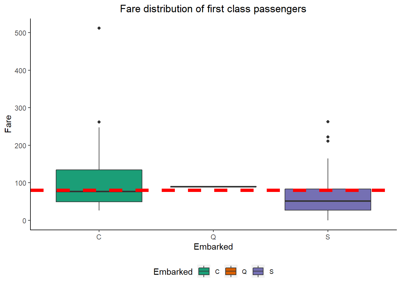
From the plot we can see that median fare for Cherbourg port passenger and the two missing embarkment feature passenger’s fare i.e. $80 concide. Therefore i am deciding to impute the missing Embarked values by the Cherbourg port.
df <- df %>%
  mutate(Embarked = ifelse(is.na(Embarked), "C", Embarked))
# Replace Embarked variable from the mice model.
#df$Embarked <- mice_output$Embarked
# Show new number of missing Embarked values
#sum(is.na(df$Embarked))Fare
df %>% filter(is.na(Fare))## # A tibble: 1 x 10
## Survived Pclass Name Sex Age SibSp Parch Ticket Fare Embarked
## <fct> <fct> <chr> <fct> <dbl> <dbl> <dbl> <chr> <dbl> <chr>
## 1 <NA> 3 Storey, Mr~ male 60.5 0 0 3701 NA 3So this male Mr.Thomas was from third class who embarked from southampton port. So let’s look at the distribution of third class passengers embarked from Southampton port.
#df$Fare <- mice_output$Fare
# Show new number of missing Fare values
#sum(is.na(df$Fare))

ggplot(filter(df, Pclass==3 & Embarked=="S"), aes(Fare)) +
  geom_density(fill="#D95F02", alpha=0.5) +
  geom_vline(aes(xintercept=median(Fare, na.rm=T)), colour='darkblue', linetype='dashed', size=2) +
  geom_vline(aes(xintercept=mean(Fare, na.rm=T)), colour='tomato', linetype='dashed', size=2) +
  ggtitle("Fare distribution of third class passengers \n embarked from Southampton port") +
  mytheme() +
  theme(plot.title = element_text(hjust = 0.5))+
  scale_fill_brewer(palette = "Dark2")
Here the mean and median are not close. The porportion of passengers with fare around median is very high whereas it is not so high around the mean. So its not good idea to impute the missing value with mean of all fares. Rather we will impute missing value with median fare of third class passengers embarked from Southampton port.
#imputing missing Fare value by median fare of third class passengers embarked from Southampton port

df <- df %>%
  mutate(Fare = ifelse(is.na(Fare), median(Fare, na.rm = TRUE), Fare))

#checking

df %>% filter(is.na(Fare))
## # A tibble: 0 x 10
## # ... with 10 variables: Survived <fct>, Pclass <fct>, Name <chr>,
## # Sex <fct>, Age <dbl>, SibSp <dbl>, Parch <dbl>, Ticket <chr>,
## # Fare <dbl>, Embarked <chr>3. Feature Engineering
Its time for feature engineering.The motive of feature engineering is to create new features which can help make predictions better. The ideas for new features usually develop during the data exploration and hypothesis generation stages.
A good approach to list all the new features that we define together in one place. We derive new feature in whole dataset.
In any data science competition the three things that distinguish winners from other in most of the cases : Feature transformation, Feature Creation and Feature Selection
Reason for transformation of data
- Some models like K-NN, SVMs, PLS, Neural networks require that the predictor variables have the same units. Centring and Scaling
the predictors can be used for this purpose.
- Other models are very sensitive to correlations between the predictors and filters or PCA Signal extraction can improve the model.
- Changing the scale of the predictors using transformation can lead to a big improvement.
- In some cases data can be encoded in a way that maximizes its effect on the model.
Preprocessing of categorical data
- Dummy Variable
Dummy variable is common technique in modelling to create numeric representation of categorical data.
There are many ways to create dummy variables in R.
Infrequent Levels in categorical factors
A zero variance predictor that has only a single value (Zero) would be the result.
Many models like linear or logistic etc. would find this numerically problematic and issue a warning and NA values for that coefficient. Trees and similar models would not notice.
Main approach to deal with this issue :-
- Run a filter on the training set predictors prior to running the model and remove zero variance predictors.
- Recode the factors so that infrequently occuring predictors are pooled into the other categories.
Since here we are trying multiple models like logistic decision tree and svm we will apply these transformation during model building process
Here we will be creating new features which will be useful in improving our accuracy of models. Also will explore it at same time.
From messy Name variable we are going to create following new features :-
- Title
- Mother
- Surname
- Solo
- FamilySize
- FamilyType
Also From Age variable we will create a new feature as stageoflife based on age group.
Title
Names has various title included we just extracted them using regular expression.
library(stringr)
df <- mutate(df, Title = str_sub(Name, str_locate(Name, ",")[,1] + 2, str_locate(Name, "\\.")[,1]-1))
df %>% group_by(Title) %>%
              summarise(count = n()) %>%
              arrange(desc(count))
## # A tibble: 18 x 2
## Title count
## <chr> <int>
## 1 Mr 757
## 2 Miss 260
## 3 Mrs 197
## 4 Master 61
## 5 Dr 8
## 6 Rev 8
## 7 Col 4
## 8 Major 2
## 9 Mlle 2
## 10 Ms 2
## 11 Capt 1
## 12 Don 1
## 13 Dona 1
## 14 Jonkheer 1
## 15 Lady 1
## 16 Mme 1
## 17 Sir 1
## 18 the Countess 1Tidy up the Title variable by adding a couple of groups and combining the other 14 titles accordingly.
df <- df %>%
          mutate(Title = factor(Title)) %>%
          mutate(Title = fct_collapse(Title, "Miss" = c("Mlle", "Ms"), "Mrs" = "Mme",
                                      "Ranked" = c( "Major", "Dr", "Capt", "Col", "Rev"),
                                      "Royalty" = c("Lady", "Dona", "the Countess", "Don", "Sir", "Jonkheer")))

ggplot(df[1:891,], aes(x = Title, fill = Survived)) +
          geom_bar(position = "fill") +
          ylab("Survival Rate") +
          geom_hline(yintercept = (sum(train$Survived)/nrow(train)), col = "white", lty = 2) +
          ggtitle("Survival Rate by Title")+
  mytheme()+
  scale_fill_brewer(palette = "Dark2")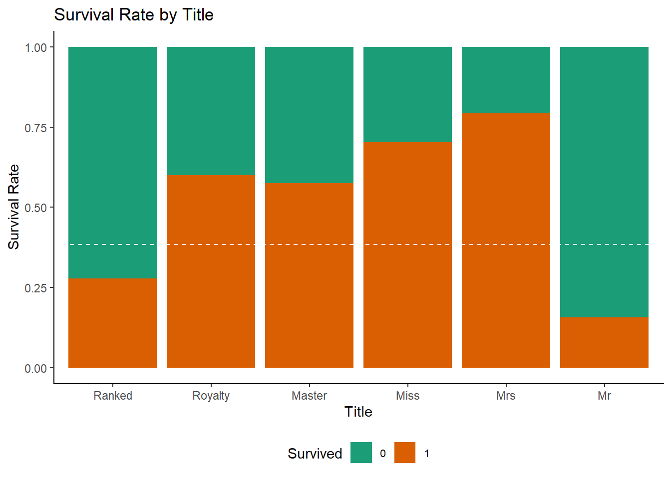
Mother Identify mothers travelling with their children, using their Title and the Parch variable
df <- df %>%
          mutate(Mother = factor(ifelse(c(df$Title == "Mrs" | df$Title == "Mme" | df$Title == "the Countess" | df$Title == "Dona" | df$Title == "Lady") & df$Parch > 0, "Yes", "No")))
ggplot(df[1:891,], aes(x = Mother, fill = Survived)) +
          geom_bar(position = "fill") +
          ylab("Survival Rate") +
          geom_hline(yintercept = (sum(train$Survived)/nrow(train)), col = "white", lty = 2) +
          ggtitle("Survival Rate by Motherhood Status")+
  mytheme()+
  scale_fill_brewer(palette = "Dark2")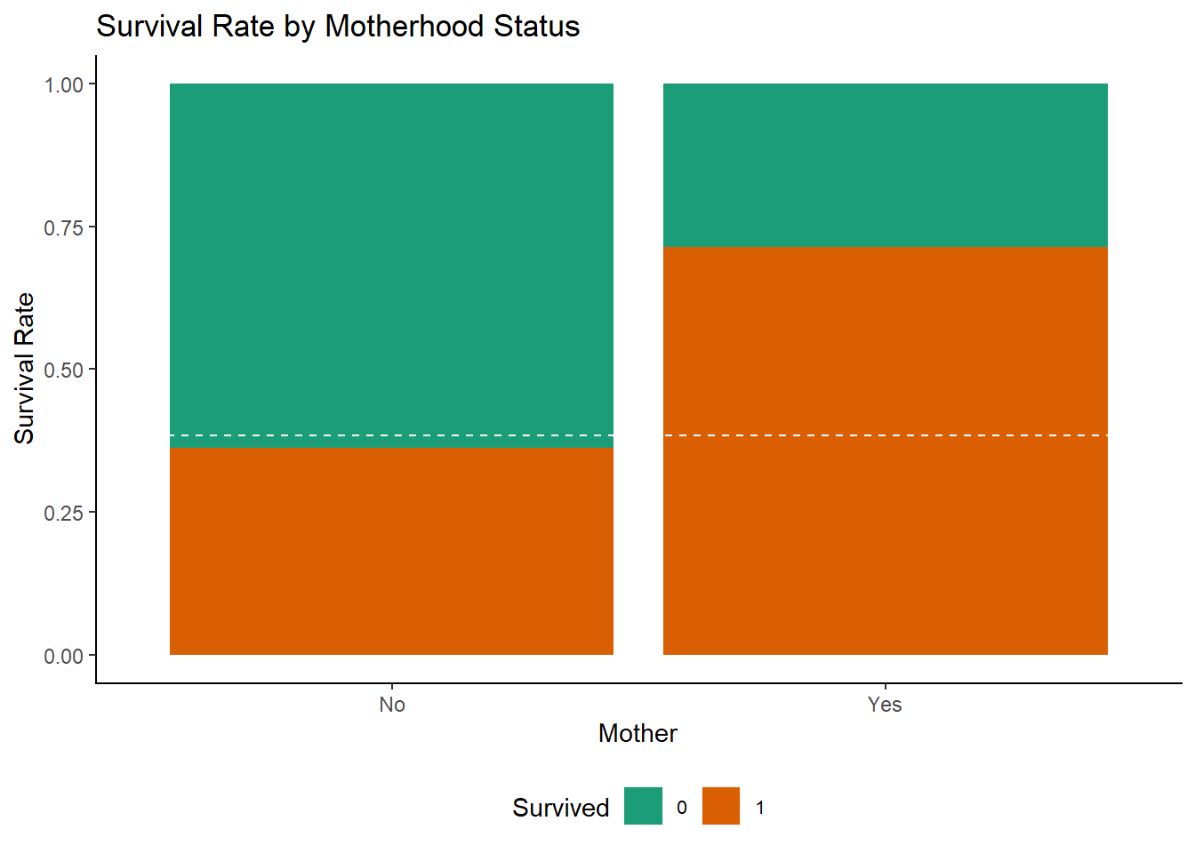
The survival chances of mothers was over twice as good as that of the other passengers.
Surname
Extracted surname from Name feature.
library(qdap)
df <- df %>%
  mutate(Surname = factor(beg2char(Name, ","))) %>%
  glimpse()
## Observations: 1,309
## Variables: 13
## $ Survived <fct> 0, 1, 1, 1, 0, 0, 0, 0, 1, 1, 1, 1, 0, 0, 0, 1, 0, 1,...
## $ Pclass <fct> 3, 1, 3, 1, 3, 3, 1, 3, 3, 2, 3, 1, 3, 3, 3, 2, 3, 2,...
## $ Name <chr> "Braund, Mr. Owen Harris", "Cumings, Mrs. John Bradle...
## $ Sex <fct> male, female, female, female, male, male, male, male,...
## $ Age <dbl> 22, 38, 26, 35, 35, 19, 54, 2, 27, 14, 4, 58, 20, 39,...
## $ SibSp <dbl> 1, 1, 0, 1, 0, 0, 0, 3, 0, 1, 1, 0, 0, 1, 0, 0, 4, 0,...
## $ Parch <dbl> 0, 0, 0, 0, 0, 0, 0, 1, 2, 0, 1, 0, 0, 5, 0, 0, 1, 0,...
## $ Ticket <chr> "A/5 21171", "PC 17599", "STON/O2. 3101282", "113803"...
## $ Fare <dbl> 7.2500, 71.2833, 7.9250, 53.1000, 8.0500, 8.4583, 51....
## $ Embarked <chr> "3", "1", "3", "3", "3", "2", "3", "3", "3", "1", "3"...
## $ Title <fct> Mr, Mrs, Miss, Mrs, Mr, Mr, Mr, Master, Mrs, Mrs, Mis...
## $ Mother <fct> No, No, No, No, No, No, No, No, Yes, No, No, No, No, ...
## $ Surname <fct> Braund, Cumings, Heikkinen, Futrelle, Allen, Moran, M...Solo
we can identify those who weren’t travelling as part of a family group.
library(see)
df <- mutate(df, Solo = factor(ifelse(SibSp + Parch + 1 == 1, "Yes", "No")))

ggplot(df[1:891,], aes(x = Solo, fill=Survived)) +
          geom_bar(position = "fill") +
          ylab("Survival Rate") +
          geom_hline(yintercept = (sum(train$Survived)/nrow(train)), col = "white", lty = 2) +
          ggtitle("Survival Rate by Solo Passenger Status")+
  mytheme()+
  scale_fill_brewer(palette = "Dark2")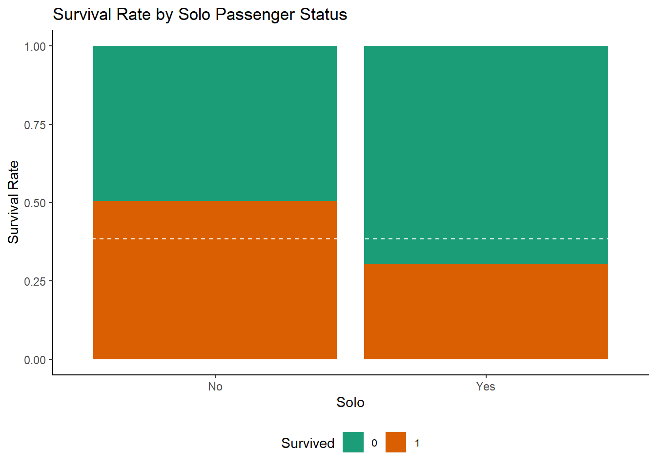
Those who weren’t part of a family group had notably worse survival chances.
Family Size and Family type :-
we can also determine family sizes using SibSp (the number of siblings/spouses aboard) and Parch.Then decided the family type based on number of people in family.
a large family as one that has more than 4 people
a medium family as one that has more than 1 but fewer than 5
single people as 1
df <- df %>%
              mutate(FamilySize = SibSp + Parch + 1) %>%
              mutate(FamilyType = factor(ifelse(FamilySize > 4, "Large", ifelse(FamilySize == 1, "Single", "Medium"))))

ggplot(df[1:891,], aes(x = FamilyType, fill = Survived)) +
          geom_bar(position = "fill") +
          ylab("Survival Rate") +
          geom_hline(yintercept = (sum(train$Survived)/nrow(train)), col = "white", lty = 2) +
          ggtitle ("Survival Rate by Family Group Size")+
  mytheme()+
    scale_fill_brewer(palette = "Dark2")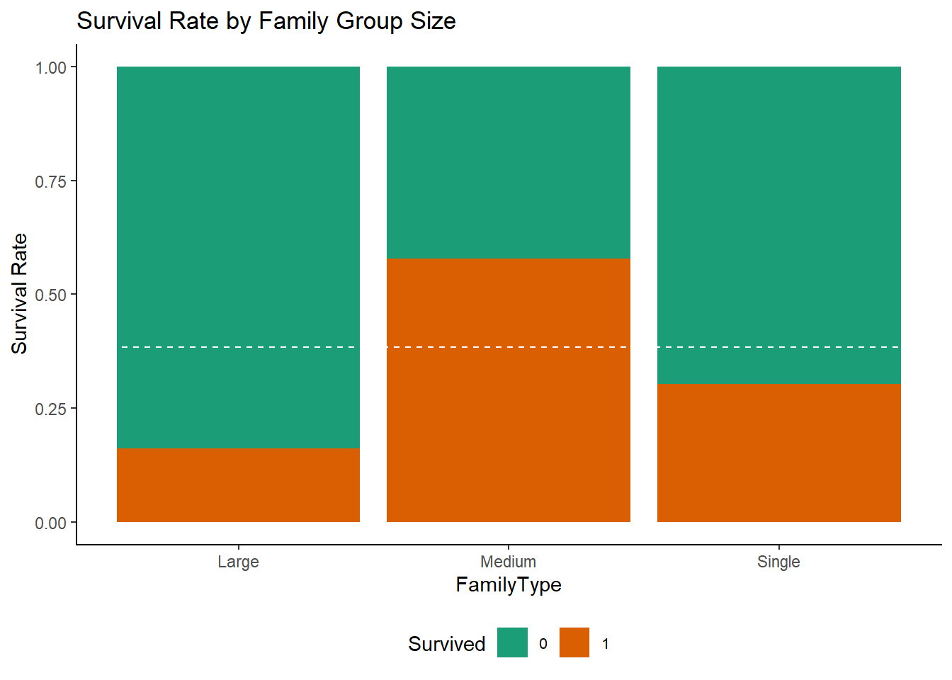
ggplot(df[1:891,], aes(x = Age, fill = Survived)) +
      geom_density(alpha = 0.4)  +
      ggtitle("Density Plot of Age related to Survival")+
  scale_fill_brewer(palette = "Dark2")+ mytheme()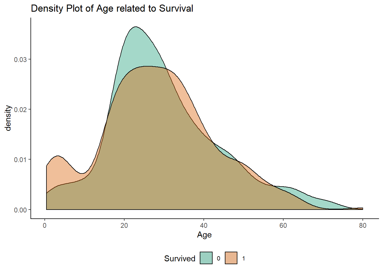
Here we see that survival rates were good up until around the age of 18, with a poor survival rate for 20-35 year olds and few survivors over the age of 60. For simplicity, let’s break this down into three groups: Child (under-18), Adult and OAP (over-60).
df <- mutate(df, LifeStage = factor(ifelse(Age < 18, "Child", ifelse(Age <= 60, "Adult", "OAP"))))

ggplot(df[1:891,], aes(x = LifeStage, fill = Survived)) +
      geom_bar(position = "fill") +
      ylab("Survival Rate") +
      geom_hline(yintercept = (sum(train$Survived)/nrow(train)), col = "white", lty = 2) +
      ggtitle("Survival Rates by Life Stage")+
   scale_fill_brewer(palette = "Dark2")+
   mytheme()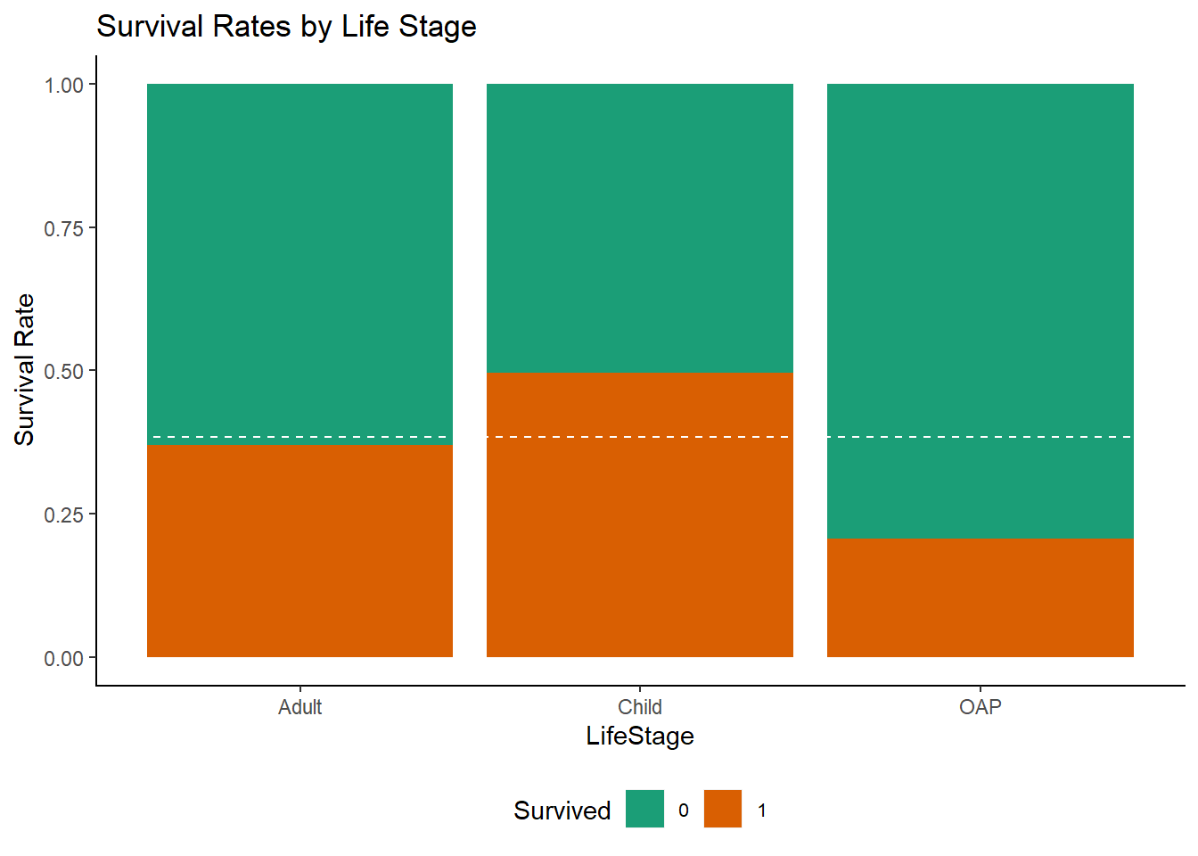
Observations from Feature engineering :-
Main reason to use feature selection :-
- Faster training
- reduces complexity of model and makes it easy for interpretation
- reduces overfitting
- it also improves the accuracy of model if right subset of feature is choosen
Next we look into different methods for feature selection.
- Filter methods
- Wrapper methods
- Embedded methods
Filter methods :-
- Generally used in preprocessing step.
- Features are selected on the basis of their scores in various statistical tests for their correlation with the outcome variable.
- Some of these test are Pearson’ Correlation, LDA, ANOVA, Chi-Square
Wrapper methods :-
Here we use to train model on subset of feature and draw inference and then we decide to add or remove features from subset. This is like a search problem and hence usually computationally expensive. Some common examples of wrapper methods are forward feature selection, backward feature elimination, recursive feature elimination, etc.
Forward Selection : Its an iterative method where we start with no feature and with each iteration we keep adding the feature which best improves are model till an addition of a new feature does not improvement performance of model.
Backward Elimination : Here we start with all the features and removes the least significant feature at each iteration which improves the performance of the model. We repeat this until no improvement is observed on removal of features.
Recursive Feature elimination : A greedy optimization algorithm which aims to find the best performing feature subset.It repeatedly creates models and keeps aside the best or the worst performing feature at each iteration. It constructs the next model with the left features until all the features are exhausted. It then ranks the features based on the order of their elimination.
One of the best ways for implementing feature selection with wrapper methods is to use Boruta package that finds the importance of a feature by creating shadow features.
To learn more about boruta package and how it works click here
Embedded Methods :-
Embedded methods combine the qualities’ of filter and wrapper methods. It’s implemented by algorithms that have their own built-in feature selection methods.
Some of the most popular examples of these methods are LASSO and RIDGE regression which have inbuilt penalization functions to reduce overfitting.
Lasso regression performs L1 regularization which adds penalty equivalent to absolute value of the magnitude of coefficients.
Ridge regression performs L2 regularization which adds penalty equivalent to square of the magnitude of coefficients.
for lasso and ridge understanding click here.*
So before moving to modelling section i drop the following features :-
- Name as i created a new feature title from it and title has more predictive power than just name.
- Ticket as i think it doesn’t have any predictive power on survival of passenger.
- Surname as it has too many levels to be used for model like random forest.
df <- select(df, -c(Name, Ticket, Surname,FamilySize)) %>%
              glimpse()
## Observations: 1,309
## Variables: 13
## $ Survived <fct> 0, 1, 1, 1, 0, 0, 0, 0, 1, 1, 1, 1, 0, 0, 0, 1, 0, ...
## $ Pclass <fct> 3, 1, 3, 1, 3, 3, 1, 3, 3, 2, 3, 1, 3, 3, 3, 2, 3, ...
## $ Sex <fct> male, female, female, female, male, male, male, mal...
## $ Age <dbl> 22, 38, 26, 35, 35, 19, 54, 2, 27, 14, 4, 58, 20, 3...
## $ SibSp <dbl> 1, 1, 0, 1, 0, 0, 0, 3, 0, 1, 1, 0, 0, 1, 0, 0, 4, ...
## $ Parch <dbl> 0, 0, 0, 0, 0, 0, 0, 1, 2, 0, 1, 0, 0, 5, 0, 0, 1, ...
## $ Fare <dbl> 7.2500, 71.2833, 7.9250, 53.1000, 8.0500, 8.4583, 5...
## $ Embarked <chr> "3", "1", "3", "3", "3", "2", "3", "3", "3", "1", "...
## $ Title <fct> Mr, Mrs, Miss, Mrs, Mr, Mr, Mr, Master, Mrs, Mrs, M...
## $ Mother <fct> No, No, No, No, No, No, No, No, Yes, No, No, No, No...
## $ Solo <fct> No, No, Yes, No, Yes, Yes, Yes, No, No, No, No, Yes...
## $ FamilyType <fct> Medium, Medium, Single, Medium, Single, Single, Sin...
## $ LifeStage <fct> Adult, Adult, Adult, Adult, Adult, Adult, Adult, Ch...Model Building
Parsnip package in action. It consist of following parts for modelling in R.
- Create Specification
- Set the engine
- Fit the model
First lets separate the datasets which we combined for eda and feature enggineering.
train <- df %>% filter(!is.na(Survived))

test <- df %>% filter(is.na(Survived))train_test_split <- initial_split(train, prop = 0.8)
titanic_train <- training(train_test_split)
titanic_test <- testing(train_test_split) Training Base Models
We will discuss below Base Models.
- Decision Tree
- Logistic Regression
- Support Vector Machine
Decision Tree model
Decision Trees are a non-parametric supervised learning method used for both classification and regression tasks. The goal is to create a model that predicts the value of a target variable by learning simple decision rules inferred from the data features.
The decision rules are generally in form of if-then-else statements. The deeper the tree, the more complex the rules and fitter the model.
To learn more about tree based models you can click here.
titanic_train## # A tibble: 713 x 13
## Survived Pclass Sex Age SibSp Parch Fare Embarked Title Mother
## <fct> <fct> <fct> <dbl> <dbl> <dbl> <dbl> <chr> <fct> <fct>
## 1 0 3 male 22 1 0 7.25 3 Mr No
## 2 1 1 fema~ 38 1 0 71.3 1 Mrs No
## 3 1 3 fema~ 26 0 0 7.92 3 Miss No
## 4 1 1 fema~ 35 1 0 53.1 3 Mrs No
## 5 0 3 male 35 0 0 8.05 3 Mr No
## 6 0 1 male 54 0 0 51.9 3 Mr No
## 7 0 3 male 2 3 1 21.1 3 Mast~ No
## 8 1 3 fema~ 27 0 2 11.1 3 Mrs Yes
## 9 1 2 fema~ 14 1 0 30.1 1 Mrs No
## 10 1 3 fema~ 4 1 1 16.7 3 Miss No
## # ... with 703 more rows, and 3 more variables: Solo <fct>,
## # FamilyType <fct>, LifeStage <fct>set.seed(1344)
titanic_train$Survived = factor(titanic_train$Survived, labels = c("no", "yes"))
titanic_test$Survived = factor(titanic_test$Survived, labels = c("no", "yes"))
model_dt <- parsnip::decision_tree(mode = "classification") %>% #Create a specification
set_engine("rpart") %>% #Set the engine
fit(as.factor(Survived) ~ ., data = titanic_train) #fit the model
model_dt## parsnip model object
##
## n= 713
##
## node), split, n, loss, yval, (yprob)
## * denotes terminal node
##
## 1) root 713 261 no (0.63394109 0.36605891)
## 2) Title=Ranked,Mr 443 67 no (0.84875847 0.15124153) *
## 3) Title=Royalty,Master,Miss,Mrs 270 76 yes (0.28148148 0.71851852)
## 6) Pclass=3 128 62 no (0.51562500 0.48437500)
## 12) Fare>=23.35 34 4 no (0.88235294 0.11764706) *
## 13) Fare< 23.35 94 36 yes (0.38297872 0.61702128)
## 26) Age>=27.5 21 8 no (0.61904762 0.38095238) *
## 27) Age< 27.5 73 23 yes (0.31506849 0.68493151) *
## 7) Pclass=1,2 142 10 yes (0.07042254 0.92957746) *Logistic Regression
Logistic Regression is a binary classification algorithm used when the response variable is dichotomous (1 or 0). Inherently, it returns the set of probabilities of target class. But, we can also obtain response labels using a probability threshold value.
But Wait we cannot simply blindly fit the logistic regression. We need to check the assumptions.Let’s check logistic regression assumption :-
- Features should be independent from each other
- Residual should not be autocorrelated
titanic_train %>% select_if(is.numeric)## # A tibble: 713 x 4
## Age SibSp Parch Fare
## <dbl> <dbl> <dbl> <dbl>
## 1 22 1 0 7.25
## 2 38 1 0 71.3
## 3 26 0 0 7.92
## 4 35 1 0 53.1
## 5 35 0 0 8.05
## 6 54 0 0 51.9
## 7 2 3 1 21.1
## 8 27 0 2 11.1
## 9 14 1 0 30.1
## 10 4 1 1 16.7
## # ... with 703 more rowscor(train[,unlist(lapply(titanic_train,is.numeric))])## Age SibSp Parch Fare
## Age 1.0000000 -0.2453464 -0.1872954 0.1034598
## SibSp -0.2453464 1.0000000 0.4148377 0.1596510
## Parch -0.1872954 0.4148377 1.0000000 0.2162249
## Fare 0.1034598 0.1596510 0.2162249 1.0000000In statistics if the correlation coefficient is either greater than 0.75 (some say 0.70 and some even say 0.8) or less than -0.75 is considered as strong correlation. We can see that sibsp and parch are highly correlated and we will drop FamilySize.
titanic_test$FamilySize <- NULL
df$FamilySize <- NULL
titanic_train$FamilySize <- NULL
#and lets check again
titanic_train %>% select_if(is.numeric) %>% cor()## Age SibSp Parch Fare
## Age 1.0000000 -0.2664636 -0.1865875 0.1020015
## SibSp -0.2664636 1.0000000 0.4253868 0.1720741
## Parch -0.1865875 0.4253868 1.0000000 0.2417257
## Fare 0.1020015 0.1720741 0.2417257 1.0000000Now none of the numeric features are strongly correlated. Hence, the Multicollinearity (a given feature in the model can be approximated by a linear combination of the other features in the model) does not exist among numeric features.
For categorical variables we will use chisquare test to test the independence of factors/categorical variables.
titanic_train %>% select_if(~!is.numeric(.)) %>% glimpse()## Observations: 713
## Variables: 9
## $ Survived <fct> no, yes, yes, yes, no, no, no, yes, yes, yes, yes, ...
## $ Pclass <fct> 3, 1, 3, 1, 3, 1, 3, 3, 2, 3, 1, 3, 3, 2, 3, 2, 3, ...
## $ Sex <fct> male, female, female, female, male, male, male, fem...
## $ Embarked <chr> "3", "1", "3", "3", "3", "3", "3", "3", "1", "3", "...
## $ Title <fct> Mr, Mrs, Miss, Mrs, Mr, Mr, Master, Mrs, Mrs, Miss,...
## $ Mother <fct> No, No, No, No, No, No, No, Yes, No, No, No, No, No...
## $ Solo <fct> No, No, Yes, No, Yes, Yes, No, No, No, No, Yes, No,...
## $ FamilyType <fct> Medium, Medium, Single, Medium, Single, Single, Lar...
## $ LifeStage <fct> Adult, Adult, Adult, Adult, Adult, Adult, Child, Ad...# Show the p-value of Chi Square tests
ps = chisq.test(titanic_train$Pclass, titanic_train$Sex)$p.value
pe = chisq.test(titanic_train$Pclass, titanic_train$Embarked)$p.value
pt = chisq.test(titanic_train$Pclass, titanic_train$Title)$p.value
pft = chisq.test(titanic_train$Pclass, titanic_train$FamilyType)$p.value
pm = chisq.test(titanic_train$Pclass, titanic_train$Mother)$p.value
pso = chisq.test(titanic_train$Pclass,titanic_train$Solo)$p.value
pls = chisq.test(titanic_train$Pclass,titanic_train$LifeStage)$p.value
se = chisq.test(titanic_train$Sex, titanic_train$Embarked)$p.value
st = chisq.test(titanic_train$Sex, titanic_train$Title)$p.value
sft = chisq.test(titanic_train$Sex, titanic_train$FamilyType)$p.value
sm = chisq.test(titanic_train$Sex, titanic_train$Mother)$p.value
sso = chisq.test(titanic_train$Sex, titanic_train$Solo)$p.value
sls = chisq.test(titanic_train$Sex, titanic_train$LifeStage)$p.value
et = chisq.test(titanic_train$Embarked, titanic_train$Title)$p.value
eft = chisq.test(titanic_train$Embarked, titanic_train$FamilyType)$p.value
em = chisq.test(titanic_train$Embarked, titanic_train$Mother)$p.value
eso = chisq.test(titanic_train$Embarked, titanic_train$Solo)$p.value
els = chisq.test(titanic_train$Embarked, titanic_train$LifeStage)$p.value
tf = chisq.test(titanic_train$Title, titanic_train$FamilyType)$p.value
tm = chisq.test(titanic_train$Title, titanic_train$Mother)$p.value
tso = chisq.test(titanic_train$Title, titanic_train$Solo)$p.value
tls = chisq.test(titanic_train$Title, titanic_train$LifeStage)$p.value
ftm = chisq.test(titanic_train$FamilyType, titanic_train$Mother)$p.value
ftso = chisq.test(titanic_train$FamilyType, titanic_train$Solo)$p.value
ftls = chisq.test(titanic_train$FamilyType, titanic_train$LifeStage)$p.value
mso = chisq.test(titanic_train$Mother, titanic_train$Solo)$p.value
mls = chisq.test(titanic_train$Mother, titanic_train$LifeStage)$p.value
sols = chisq.test(titanic_train$Solo, titanic_train$LifeStage)$p.value
cormatrix = matrix(c(0, ps, pe, pt, pft, pm, pso, pls,
ps, 0, se, st, sft, sm, sso, sls,
pe, se, 0, et, eft, em, eso, els,
pt, st, et, 0, tf, tm, tso, tls,
pft,sft, eft, tf, 0, ftm, ftso, ftls,
pm, sm, em, tm, ftm, 0, mso, mls,
pso,sso, eso,tso, ftso, mso, 0, sols,
pls,sls, els,tls, ftls, mls, sols, 0),
8, 8, byrow = TRUE)
row.names(cormatrix) = colnames(cormatrix) = c("Pclass", "Sex", "Embarked", "Title", "FamilyType", "Mother", "Solo", "LifeStage")
cormatrix## Pclass Sex Embarked Title
## Pclass 0.000000e+00 7.933846e-05 1.096579e-19 4.540254e-11
## Sex 7.933846e-05 0.000000e+00 3.750507e-05 1.134004e-150
## Embarked 1.096579e-19 3.750507e-05 0.000000e+00 2.994070e-06
## Title 4.540254e-11 1.134004e-150 2.994070e-06 0.000000e+00
## FamilyType 6.534996e-10 6.505002e-16 4.429834e-05 1.802722e-47
## Mother 1.408353e-01 2.535110e-21 7.746134e-01 5.178247e-63
## Solo 1.246114e-03 1.227681e-16 7.775292e-03 1.014950e-38
## LifeStage 4.911776e-07 2.079754e-04 3.156886e-02 6.382941e-48
## FamilyType Mother Solo LifeStage
## Pclass 6.534996e-10 1.408353e-01 1.246114e-03 4.911776e-07
## Sex 6.505002e-16 2.535110e-21 1.227681e-16 2.079754e-04
## Embarked 4.429834e-05 7.746134e-01 7.775292e-03 3.156886e-02
## Title 1.802722e-47 5.178247e-63 1.014950e-38 6.382941e-48
## FamilyType 0.000000e+00 9.310864e-17 1.492854e-155 4.240195e-26
## Mother 9.310864e-17 0.000000e+00 3.574522e-17 5.509061e-02
## Solo 1.492854e-155 3.574522e-17 0.000000e+00 6.396836e-19
## LifeStage 4.240195e-26 5.509061e-02 6.396836e-19 0.000000e+00Since all the p-values < 0.05, we reject each Ho:Two factors are independent at 5% significance level and indeed at any reasonable level of significance. This violates the independence assumption of features and can be confirmed that multicollinearity does exist among factors.
We will deal with this issue later.
model_log<- parsnip::logistic_reg(mode = "classification") %>%
  set_engine("glm") %>%
  fit(formula = Survived~.,
                data = mutate(titanic_train, Survived= factor(Survived, labels = c("no", "yes"))))

model_log
## parsnip model object
##
##
## Call: stats::glm(formula = formula, family = stats::binomial, data = data)
##
## Coefficients:
## (Intercept) Pclass2 Pclass3 Sexmale
## 14.250542 -1.454999 -2.395267 -16.326923
## Age SibSp Parch Fare
## -0.020733 -0.204633 -0.014102 0.001747
## Embarked2 Embarked3 EmbarkedC TitleRoyalty
## -0.056638 -0.355190 12.839950 0.205453
## TitleMaster TitleMiss TitleMrs TitleMr
## 4.538363 -12.616712 -12.378551 0.604535
## MotherYes SoloYes FamilyTypeMedium FamilyTypeSingle
## 0.070144 2.268958 2.010797 NA
## LifeStageChild LifeStageOAP
## -0.074196 -0.666036
##
## Degrees of Freedom: 712 Total (i.e. Null); 692 Residual
## Null Deviance: 936.6
## Residual Deviance: 553.5 AIC: 595.5To learn more about logistic regression click here.
Support Vector Machine
Support Vector Machine (SVM) is a supervised machine learning algorithm which can be used for both classification or regression challenges. However, it is mostly used in classification problems. In this algorithm, we plot each data item as a point in n-dimensional space (where n is number of features you have) with the value of each feature being the value of a particular coordinate. Then, we perform classification by finding the hyper-plane that differentiate the two classes very well.
To learn more about SVM click here
model_svm<- parsnip::svm_poly(mode = "classification") %>%
  set_engine("kernlab") %>%
  fit(formula = Survived~.,
                data = mutate(titanic_train, Survived= factor(Survived, labels = c("no", "yes"))))
## Setting default kernel parametersmodel_svm## parsnip model object
##
## Support Vector Machine object of class "ksvm"
##
## SV type: C-svc (classification)
## parameter : cost C = 1
##
## Polynomial kernel function.
## Hyperparameters : degree = 1 scale = 1 offset = 1
##
## Number of Support Vectors : 307
##
## Objective Function Value : -241.1986
## Training error : 0.168303
## Probability model included.titanic_train$Survived = factor(titanic_train$Survived, labels = c("no", "yes"))
titanic_test$Survived = factor(titanic_test$Survived, labels = c("no", "yes"))
predictions_dt <-tibble(
actual = titanic_test$Survived,
predicted_dt = predict(model_dt,titanic_test, type = "class") %>% pull(.pred_class)
)
predictions_log <-tibble(
actual = titanic_test$Survived,
predicted_log = predict(model_log,titanic_test, type = "class") %>% pull(.pred_class)
)
predictions_svm <-tibble(
actual = titanic_test$Survived,
predicted_svm = predict(model_svm,titanic_test, type = "class") %>% pull(.pred_class)
)The yardstick package is a tidy interface for computing measure of performances.
The individual functions for specific metrics (e.g. accuracy(), rmse() etc.)
When more than one metric is desired metric_set() can create a new function that wraps them.
dt <- yardstick::metrics(predictions_dt, actual, predicted_dt) %>%  mutate(model_type = "decision_tree") %>% select(model_type, everything(),-.estimator)
log <- yardstick::metrics(predictions_log, actual, predicted_log) %>% mutate(model_type = "logistic_regression") %>% select(model_type, everything(), -.estimator)
svm <- yardstick::metrics(predictions_svm, actual, predicted_svm) %>% mutate(model_type = "svm")%>% select(model_type, everything(), -.estimator)

rbind(dt,log,svm) %>% spread(.metric, .estimate)
## # A tibble: 3 x 3
## model_type accuracy kap
## <chr> <dbl> <dbl>
## 1 decision_tree 0.803 0.597
## 2 logistic_regression 0.798 0.591
## 3 svm 0.815 0.624Observations :-
- Among three different types of classification models used decision tree gave the best results in terms of accuracy.
- Next we will try with ensemble model techniques to improve our results further.
dt_probs<- model_dt %>%
  predict(titanic_test, type = "prob") %>%
  bind_cols(titanic_test)
dt_probs %>% glimpse()
## Observations: 178
## Variables: 15
## $ .pred_no <dbl> 0.84875847, 0.84875847, 0.61904762, 0.84875847, 0.8...
## $ .pred_yes <dbl> 0.1512415, 0.1512415, 0.3809524, 0.1512415, 0.15124...
## $ Survived <fct> no, no, yes, no, no, no, no, yes, yes, no, no, yes,...
## $ Pclass <fct> 3, 3, 3, 3, 2, 1, 3, 3, 1, 1, 1, 3, 2, 3, 1, 3, 3, ...
## $ Sex <fct> male, male, female, male, male, male, female, femal...
## $ Age <dbl> 19.0, 20.0, 43.0, 16.0, 66.0, 28.0, 40.0, 18.0, 26....
## $ SibSp <dbl> 0, 0, 0, 0, 0, 1, 1, 0, 0, 1, 0, 1, 0, 5, 0, 3, 1, ...
## $ Parch <dbl> 0, 0, 0, 0, 0, 0, 0, 0, 0, 0, 0, 1, 0, 2, 0, 0, 3, ...
## $ Fare <dbl> 8.4583, 8.0500, 7.2250, 7.8958, 10.5000, 82.1708, 9...
## $ Embarked <chr> "2", "3", "1", "3", "3", "1", "3", "2", "3", "3", "...
## $ Title <fct> Mr, Mr, Mrs, Mr, Mr, Mr, Mrs, Miss, Mr, Mr, Mr, Mas...
## $ Mother <fct> No, No, No, No, No, No, No, No, No, No, No, No, No,...
## $ Solo <fct> Yes, Yes, Yes, Yes, Yes, No, No, Yes, Yes, No, Yes,...
## $ FamilyType <fct> Single, Single, Single, Single, Single, Medium, Med...
## $ LifeStage <fct> Adult, Adult, Adult, Child, OAP, Adult, Adult, Adul...ROC-Curve
dt_probs %>%
  roc_curve(Survived, .pred_no) %>%
  autoplot()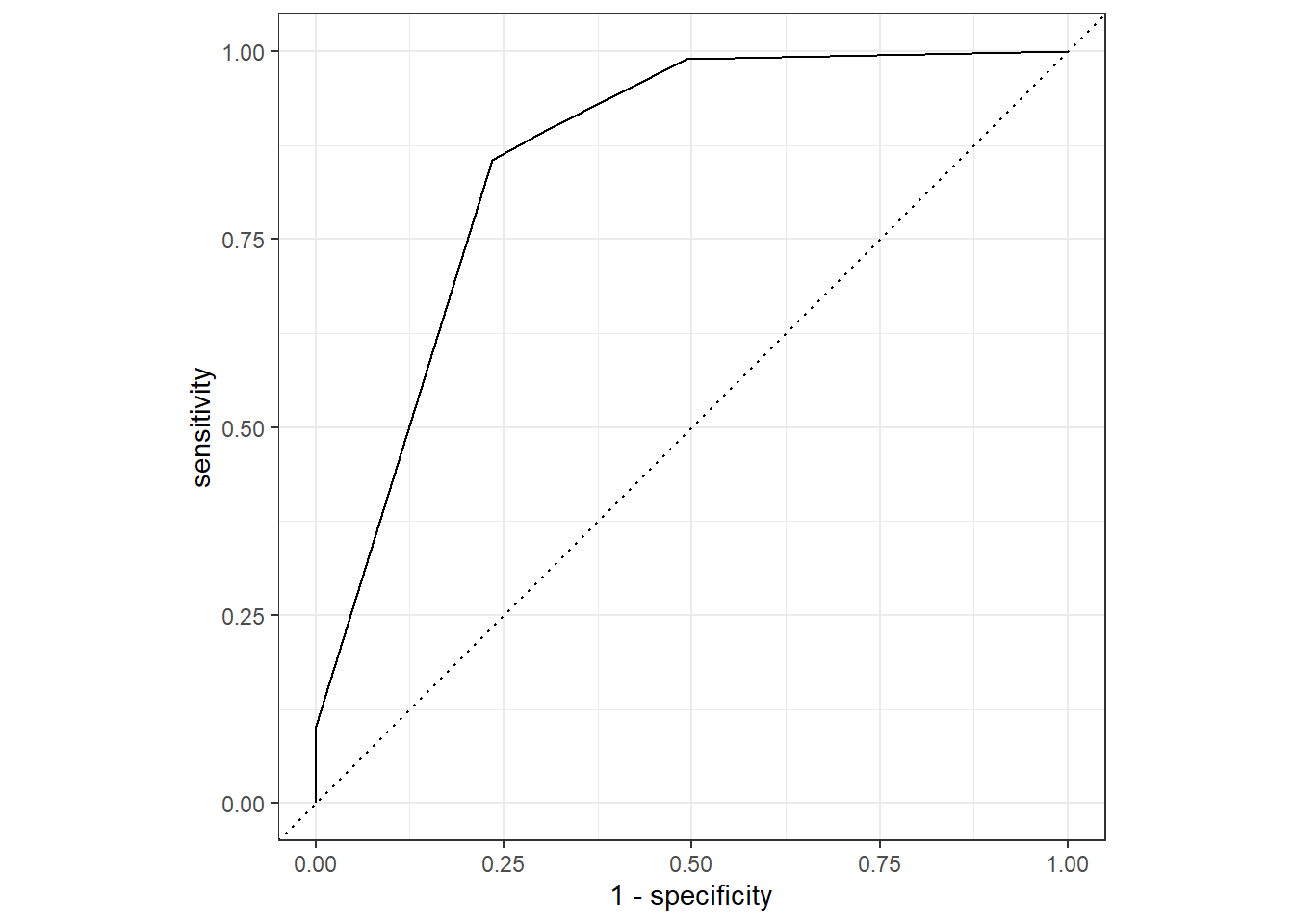
In next blog post we will learn about :-
- Resampling techniques to get better idea of our model performance
- Ensemble modelling techniques to improve our model performance
- Interpretating machine learning models
